
I. Intro
You can use search functions to search for data in Lark Sheets and process data more efficiently. For example, you can use the COLUMN function to return the column number of a cell.
II. Supported search functions
III. How to use search functions
CHOOSECOLS function
Use the CHOOSECOLS function to create an array from specified columns.
- Formula: =CHOOSECOLS(array, col_num1, [col_num2], ...).
- Arguments:
- array: The array or cell range containing the columns to be returned (for example, A2:B9).
- col_num1: The first column to be returned. For example, if you enter 2, the data in column 2 of A2:B9 will be returned.
- col_num2: Additional columns to be returned (optional).
Note: Enter a negative column number to count from the right of the specified array.
- For example, you can use the CHOOSECOLS function to extract data from non-adjacent columns. In the following example, you can use CHOOSECOLS(A1:D7,1,2) to extract each student's name and their corresponding Chinese language score. A1:D7 denotes the data range, 1 denotes column 1, and 2 denotes column 2.
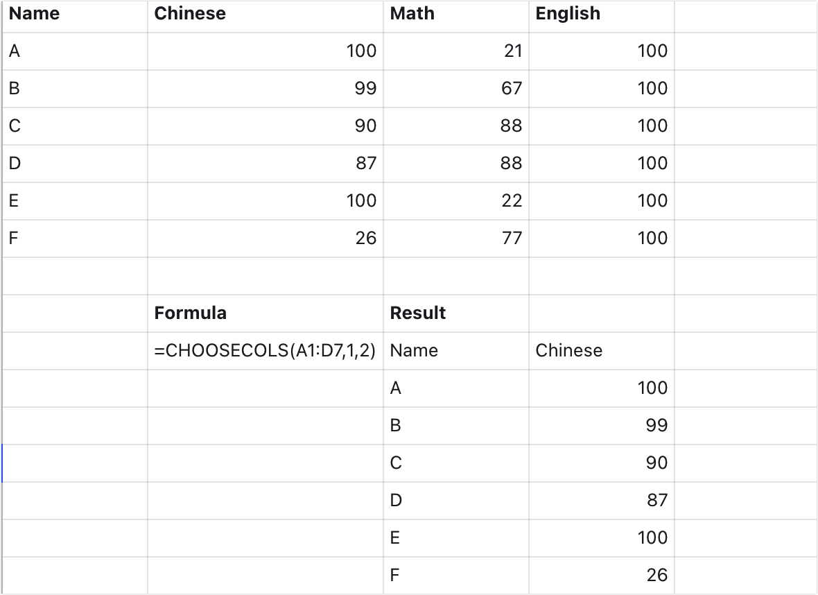
250px|700px|reset
CHOOSEROWS function
Use the CHOOSEROWS function to create an array from specified rows.
- Formula: =CHOOSEROWS(array, row_num1, [row_num2], ...)
- Arguments:
- array: The array or cell range containing the rows to be returned (for example, A2:B9).
- row_num1: The first row to be returned. For example, if you enter 2, the data in row 2 of A2:B9 will be returned.
- row_num2: Additional rows to be returned (optional).
Note: Enter a negative row number to count from the bottom of the specified array.
- For example, you can use the CHOOSEROWS function to extract data from specific rows. In the following example, you can use CHOOSEROWS(A1:D7,2,3) to extract the exam scores of students A and B. A1:D7 denotes the data range, 2 denotes row 2, and 3 denotes row 3.
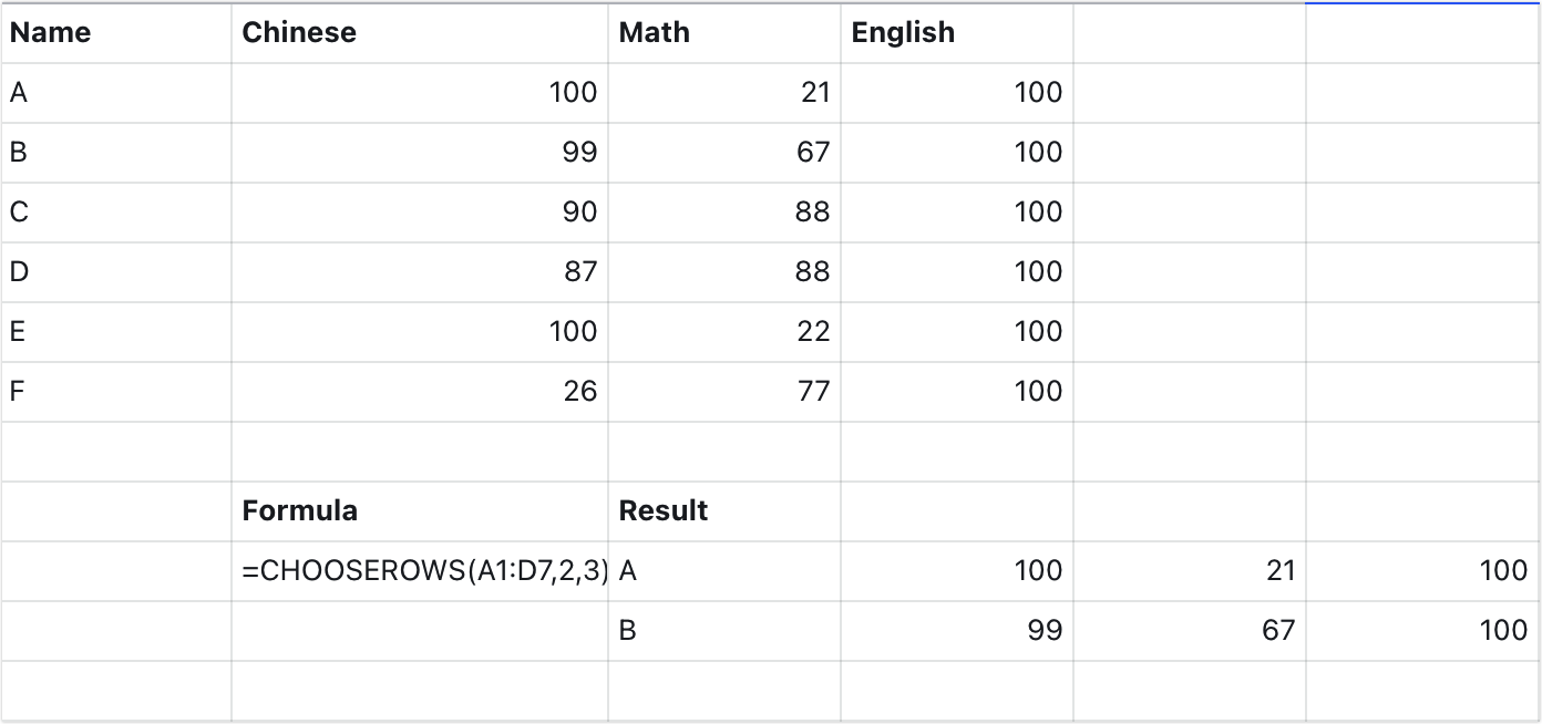
250px|700px|reset
COLUMNS function
Use the COLUMNS function to determine the number of columns in a specified array or range.
- Formula: COLUMNS(range)
- Arguments:
- range: The array or range whose column count will be returned (for example, B1:D7).
- For example, you can use the COLUMNS function to determine the number of columns in a spreadsheet. In the following example, you can use COLUMNS(B1:D7) to calculate the number of subjects in a spreadsheet of exam scores. B1:D7 denotes the range whose column count you want to calculate.
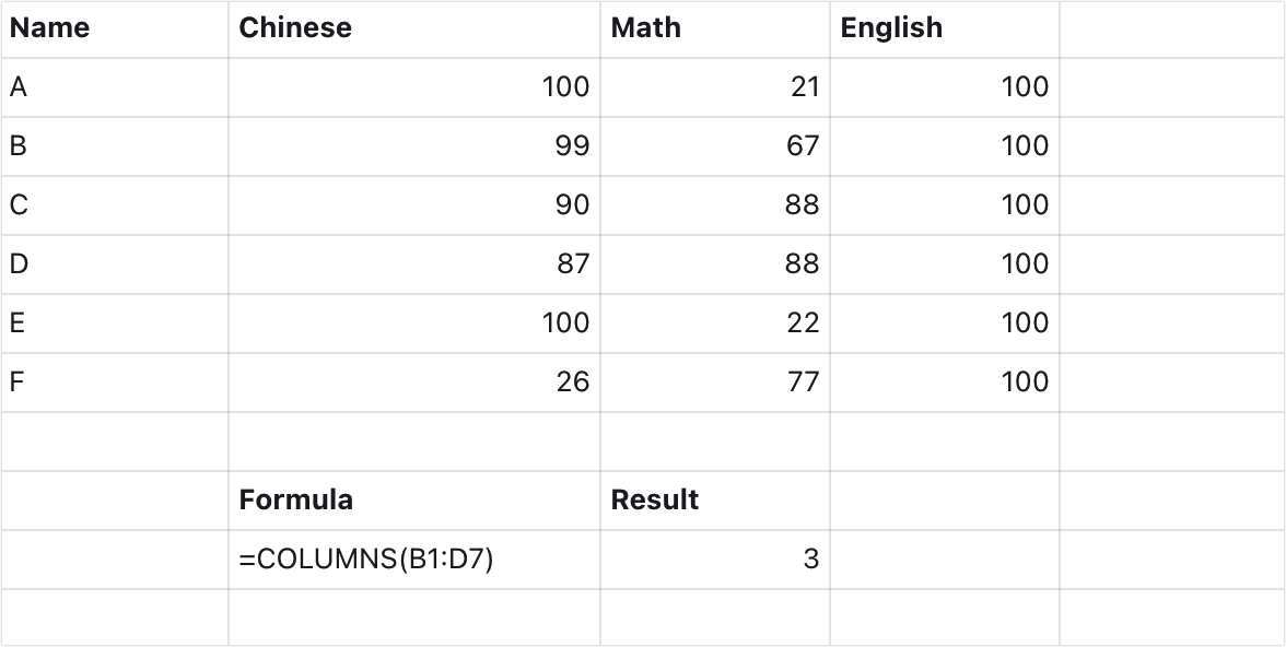
250px|700px|reset
DROP function
Use the DROP function to exclude a specified number of rows or columns from the beginning or end of an array.
- Formula: DROP(array, rows, [columns])
- Arguments:
- array: The array or range from which to exclude rows or columns (for example, A1:D7).
- rows: The number of rows to exclude. For example, 1 denotes that the first row of data will be dropped from A1:D7.
- columns: Optional. The number of columns to drop. For example, 1 denotes that the first column of data will be dropped from A1:D7.
Note: A negative value for rows or columns drops from the end of the array.
- For example, you can use the DROP function to exclude the heading and only return the data. In the following example, you can use =DROP(A1:D7,1) to exclude the heading from a sheet of exam scores.
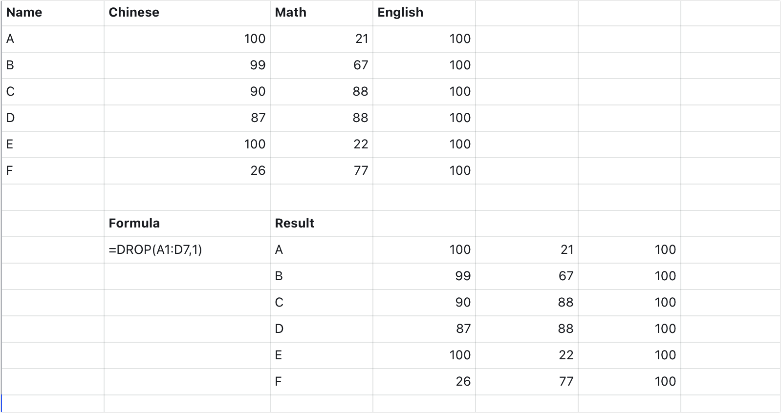
250px|700px|reset
EXPAND function
Use the EXPAND function to expand or pad an array to specified rows and columns.
- Function: EXPAND(array, rows, [columns], [pad_with])
- Arguments:
- array: The array or range to expand (for example, A2:B3).
- rows: The number of rows in the expanded array. For example, 3 denotes that the array will be expanded to 3 rows of data.
- columns: Optional. The number of columns in the expanded array. For example, 3 denotes that the array will be expanded to 3 columns of data.
- pad_with: Optional. The value with which to pad when the element is empty. The default is #N/A.
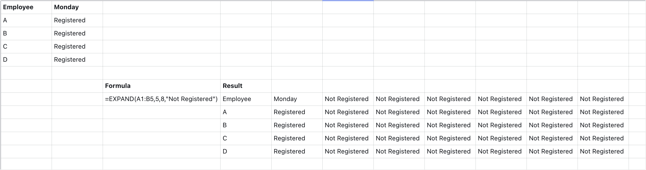
- For example, you can use the EXPAND function to quickly expand a set of data. In the following example, you can use EXPAND(A1:B5,5,8, "Not Registered") to expand the data in a sign-up sheet. After making a few simple edits, you can complete sign-up records for the whole week.
250px|700px|reset
HSTACK function
Use the HSTACK function to merge different ranges of data horizontally.
- Formula: HSTACK(range1; [range2, …])
- Arguments:
- range1: The array or range to append (for example, A2:F9).
- range2: Optional. Additional ranges to add to range1.
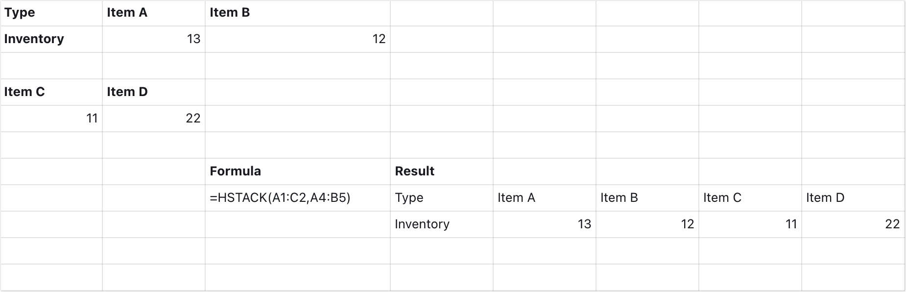
- For example, you can use the HSTACK function to quickly append data. In the following inventory sheet, you can use HSTACK(A1:C2,A4:B5) to horizontally merge data in A1:C2 and A4:B5.
250px|700px|reset
SORTBY
Use the SORTBY function to sort a range or array based on the values in a corresponding range or array.
- Formula: SORTBY(array, by_array1, [sort_order1], [by_array2, sort_order2],…)
- Arguments:
- array: The array or range to sort (for example, A2:C20).
- by_array1: The array or range to sort by. For example, A2:A20 denotes that the data should be sorted by column A.
- sort_order1: Optional. The order to use for sorting. 1 denotes ascending, and -1 denotes descending. The default order is ascending.
- by_array2: Optional. Additional arrays or ranges to sort by. When there are two or more equal values in the first column, these values will be sorted according to the second column, and so on.
- sort_order2: Additional orders to use for sorting (optional).
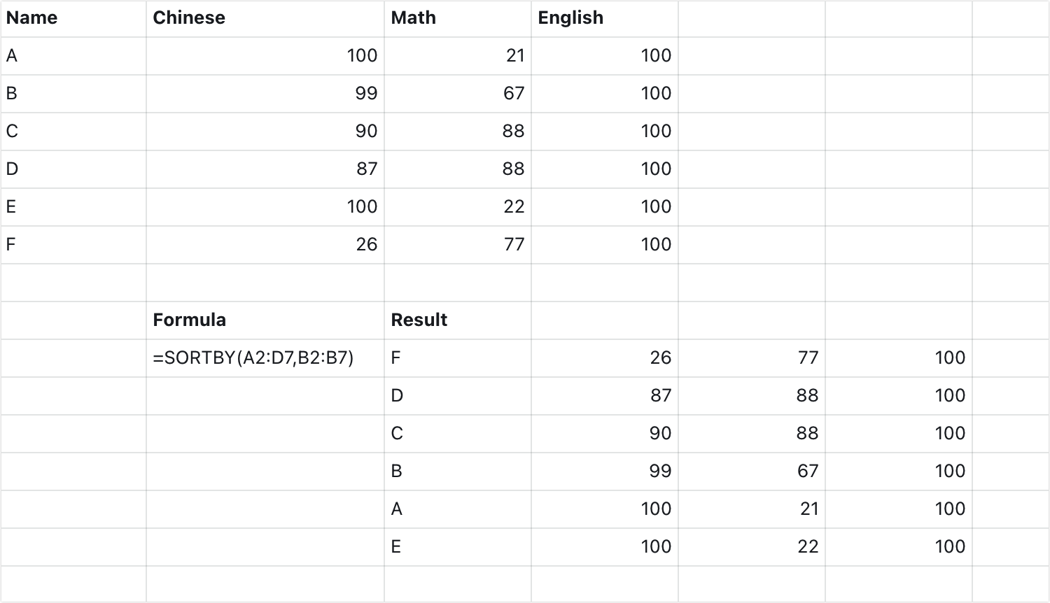
- For example, you can use the SORTBY function to sort a set of data. In the following example, you can use SORTBY(A2:D7,B2:B7) to sort students by their Chinese exam scores.
250px|700px|reset
SORTN function
Use the SORTN function to obtain the first n items in a sorted data set.
- Formula: SORTN(array, [n], [display_ties_mode], [sort_column, ...], [is_ascending], ...)
- Arguments:
- array: The array or range to sort (for example, A2:C20).
- n: Optional. The number of items to return. For example, if you enter 2, the first two values will be returned after sorting. n must be greater than 0. If no value is entered, all values will be returned.
- display_ties_mode: Optional. Determines how identical values are displayed. 0 means return all identical values, 1 means return only the first identical value, and 2 means return only the last identical value. If no value is entered, all identical values will be returned.
- sort_column: Optional. The column to sort by. For example, 1 denotes that the data should be sorted by the first column. If no value is entered, the data will be sorted by the first column.
- is_ascending: Optional. The order to use for sorting. False denotes ascending, and True denotes descending. The default order is ascending.
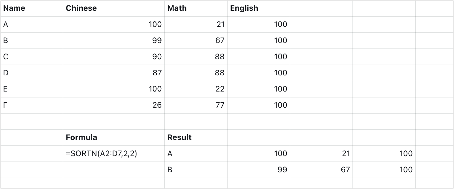
- For example, you can use the SORTN function to quickly filter the first n values that meet specified conditions. In the following example, you can use SORTN(A2:D7,2,2) to filter the scores for the two top-performing students in the Chinese exam.
250px|700px|reset
TAKE function
Use the TAKE function to obtain a specified number of contiguous rows or columns from the start or end of an array.
- Formula: TAKE(array, rows,[columns])
- Arguments:
- array: The array or range from which to take rows or columns (for example, A2:C4).
- rows: The number of rows to take. For example, 2 denotes take the first two rows.
- columns: Optional. The number of columns to take. If no value is entered, all columns will be returned.
Note: A negative value for rows or columns takes from the end of the array.
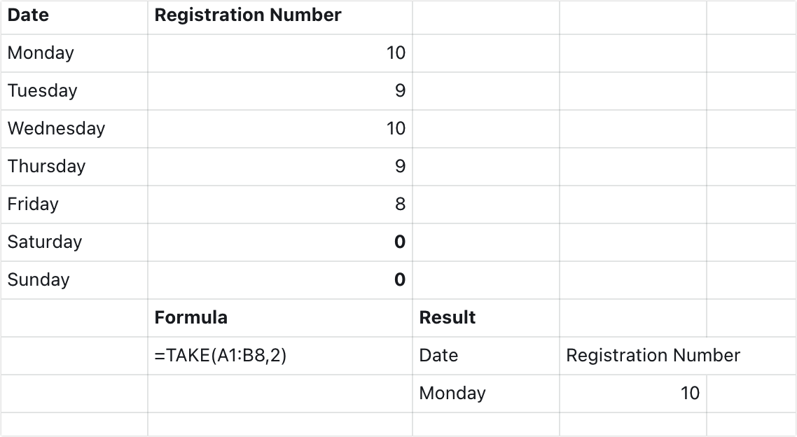
- For example, you can use the TAKE function to quickly obtain data from a specified number of rows or columns. In the following example, you can use TAKE(A1:B8,2) to obtain the data from the first two rows in an attendance sheet.
250px|700px|reset
TOCOL function
Use the TOCOL function to transform an array into a single column.
- Formula: TOCOL(array_or_range, [ignore], [scan_by_column])
- Arguments:
- array_or_range: The array or range to transform into a column (for example, A2:F9).
- ignore: Optional. The data to be ignored. You can specify one or more types of data. 0 means retain all values, 1 means ignore empty cells, 2 means ignore error values, and 3 means ignore other empty cells and error values. If no value is entered, all values will be retained.
- scan_by_column: Optional. Determines how the array is scanned. Enter True to scan the array by column, or False to scan the array by row. By default, the array is scanned by row.
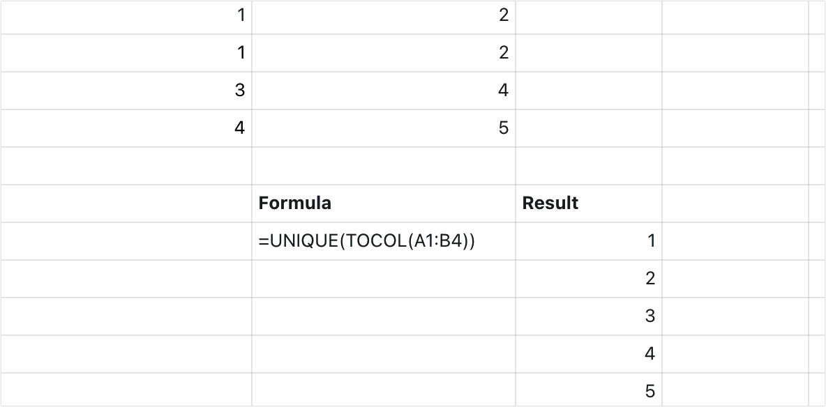
- For example, you can use the TOCOL function to quickly transform several columns of data into one column. In the following example, you can use TOCOL(A2:B5,1,FALSE) to transform the data in A2:B5 into one column. You can also use the UNIQUE function to avoid duplicate data.
250px|700px|reset
TOROW function
Use the TOROW function to transform an array into a single row.
- Formula: TOROW(array_or_range, [ignore], [scan_by_column])
- Arguments:
- array_or_range: The array or range to transform into a column (for example, A2:F9).
- ignore: Optional. The data to be ignored. You can specify one or more types of data. 0 means retain all values, 1 means ignore empty cells, 2 means ignore error values, and 3 means ignore other empty cells and error values. If no value is entered, all values will be retained.
- scan_by_column: Optional. Determines how the array is scanned. Enter True to scan the array by column, or False to scan the array by row. By default, the array is scanned by row.
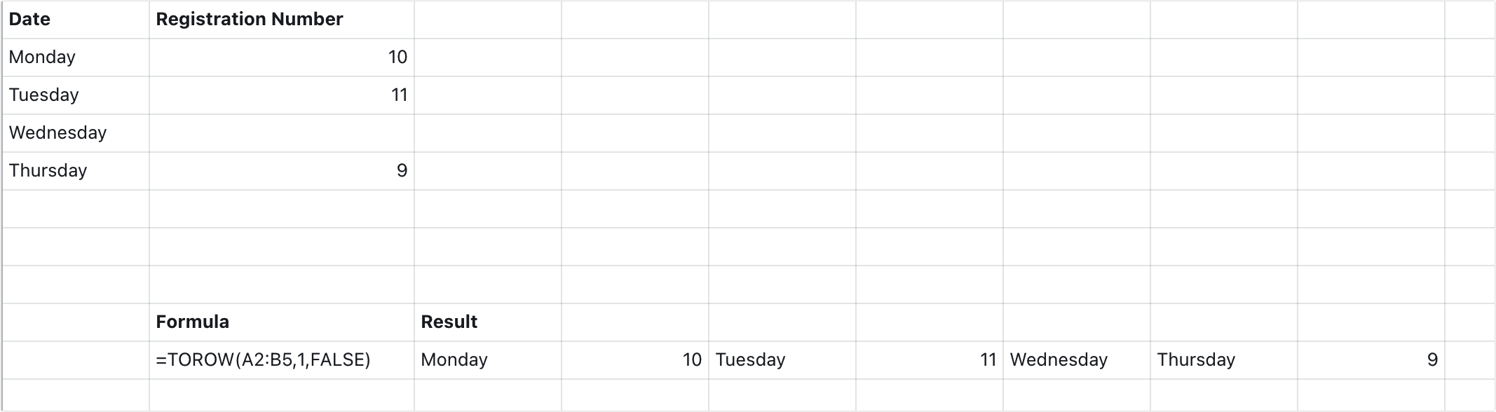
- For example, you can use the TOROW function to quickly transform several columns of data into one row. In the following example, you can use TOROW(A2:B5,1,FALSE) to transform the data.
250px|700px|reset
VSTACK function
Use the VSTACK function to merge different ranges of data vertically.
- Formula: VSTACK(range1; [range2, …])
- Arguments:
- range1: The array or range to merge (for example, A2:F9).
- range2: Additional ranges to add to range1 (optional).
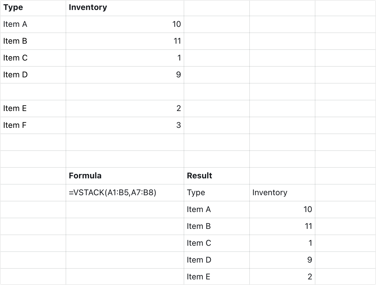
- For example, you can use the VSTACK function to quickly merge data. In the following inventory sheet, you can use VSTACK(A1:B5,A7:B8) to vertically merge data in A1:B5 and A7:B8.
250px|700px|reset
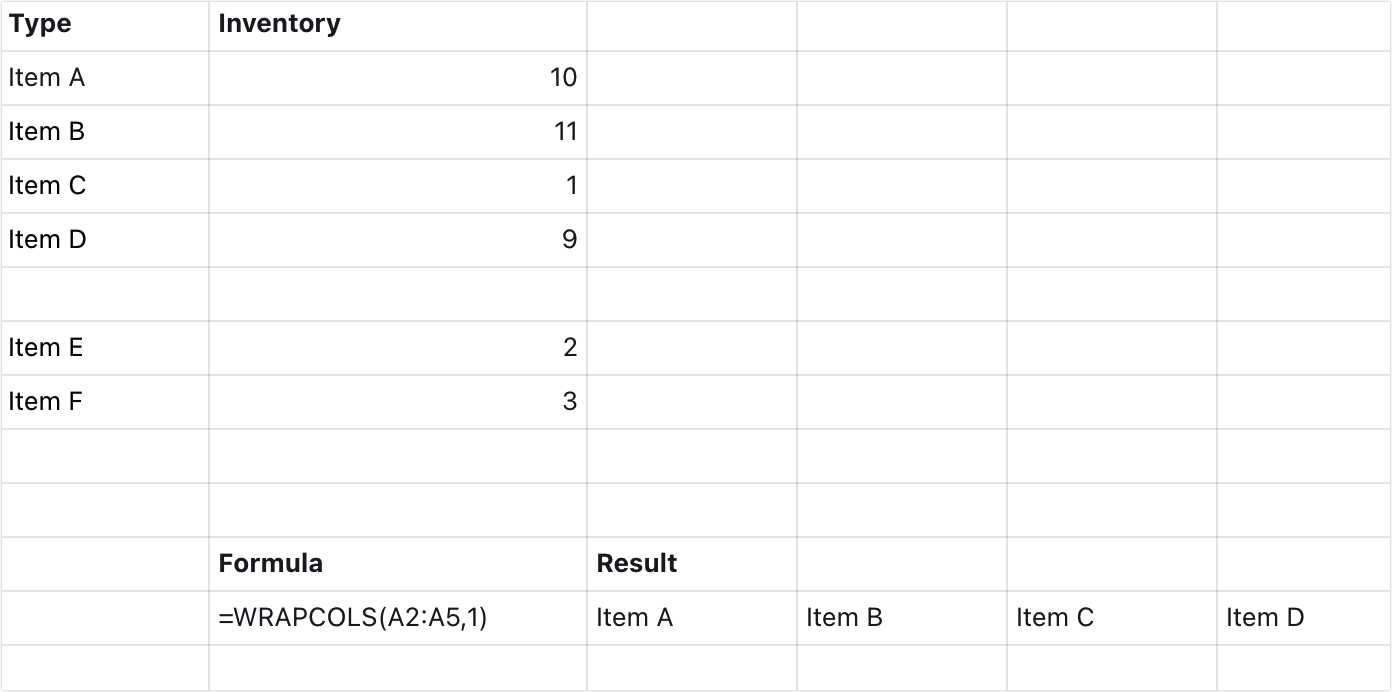
WRAPCOLS function
Use the WRAPCOLS function to wrap a range of data by columns with a specified number of cells.
- Formula: WRAPCOLS(range, wrap_count, [pad_with])
- Arguments:
- range: The array or range to wrap (for example, A2:A9). Must be a single row or column.
- wrap_count: The maximum number of rows for each column. For example, if you enter 2, each column will display a maximum of two rows of data.
- pad_with: Optional. The value with which to fill the empty cells in the range. By default, empty cells are filled with #N/A.
- For example, you can use the WRAPCOLS function to wrap data in a single column into multiple columns. In the following example, you can use WRAPCOLS(A2:A5,1) to display the data in A2:A9 in an array of 1 row per column.
250px|700px|reset
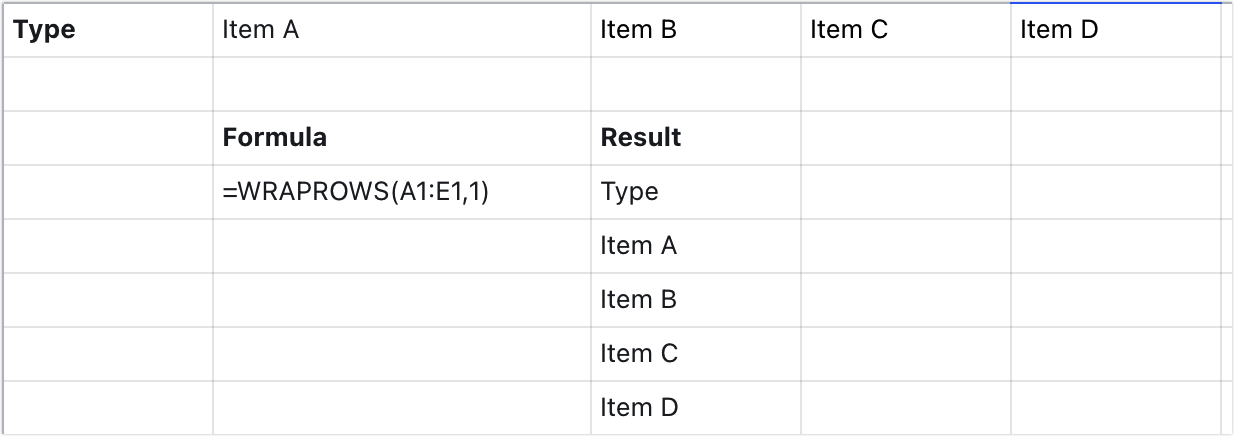
WRAPROWS function
Use the WRAPROWS function to wrap a range of data by rows with a specified number of columns.
- Formula: WRAPROWS(range, wrap_count, [pad_with])
- Arguments:
- range: The array or range to wrap (for example, A2:A9). Must be a single row or column.
- wrap_count: The maximum number of columns for each row. For example, if you enter 2, each row will display a maximum of two columns of data.
- pad_with: Optional. The value with which to fill the empty cells in the range. By default, empty cells are filled with #N/A.
- For example, you can use the WRAPROWS function to wrap data in a single row into multiple rows. In the following example, you can use WRAPROWS(A1:E1,1) to display the data in A1:E1 in an array of 1 column per row.
250px|700px|reset
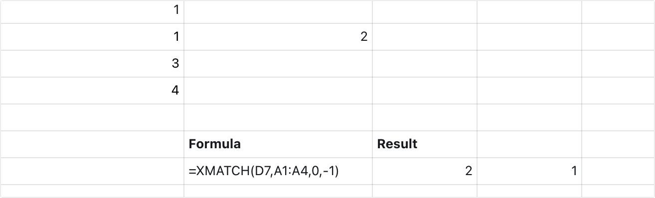
XMATCH function
Use the XMATCH function to search for a specified item in an array or range of cells, and then return the item's relative position.
- Formula: XMATCH(search_key, lookup_range, [match_mode], [search_mode])
- Arguments:
- search_key: The value you want to find. For example, F2 means the function will search for the value in cell F2.
- lookup_range: The array or range in which to look for values (for example, C3:C9). Must be a single row or column.
- match_mode: Optional. Enter 0 for an exact match, 1 for an exact match or the next value that's greater, or -1 for an exact match or the next value that's lower. By default, the function will search for an exact match.
- search_mode: Optional. Enter 1 to search from the first entry to the last, or -1 to search from the last entry to the first.
- For example, you can use the XMATCH function to quickly find the relative position of a value in a data range. In the following example, you can use XMATCH(D7,A1:A4,0,-1) to find the relative position of the D7 value in A1:A4.
250px|700px|reset
IV. FAQs