
I. Intro
The ADDRESS function can be used to obtain the cell address corresponding to the specified row number and column number in a sheet. For example, ADDRESS(1,2) returns the cell address of the first row and the second column, which is $B$1.
II. About the function
- Formula: = ADDRESS(row, column, [absolute_relative_mode], [use_a1_notation], [sheet])
- Arguments:
- row: The row number of the cell address to be obtained.
- column: The column number of the cell address to be obtained.
- absolute_relative_mode: Optional. Specifies the reference mode used by the returned cell address.
Value | Address reference mode | Return value example |
1 or omitted | Both row number and column number are absolute values | $B$1 |
2 | Row number is absolute value, column number is relative value | $B1 |
3 | Row number is relative value, column number is absolute value | B$1 |
4 | Both row number and column number are relative values | B1 |
- use_a1_notation: Optional. Specifies the coordinate mode used by the returned cell address.
- TRUE or omitted: Specifies the reference style as A1, where columns are represented by letters, and rows are represented by numbers. For example, the cell in the first row and first column is written as "A1".
- FALSE: Specify the reference style as R1C1, that is, columns are represented by C (Column), and rows are represented by R (Row). For example, the cell in the first row and first column is written as "R1C1".
- sheet: Optional. Specifies the sheet where the cell is located. You need to fill in the name of the sheet and enclose it in double quotation marks (for example: "Sheet1"). If the cell and the formula are on the same sheet, you can omit this argument.
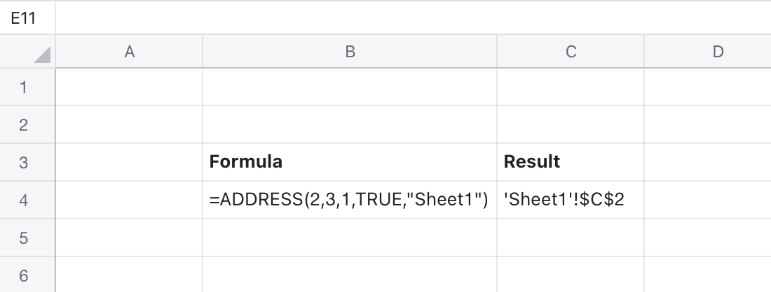
- Example: =ADDRESS(2,3,1,TRUE,"Sheet1") returns the cell address of the second row and the first column in Sheet1. The address is a relative address and is represented in A1 style as 'Sheet1'!$C$2.
- Note: If you need to omit an argument in the middle of the formula, add commas to indicate the use of the default values. For example, if you want to omit the 3rd and 4th arguments in the formula above, you need to add two commas and write the formula as =ADDRESS(2,3,,,"Sheet1").
250px|700px|reset
III. Steps
Use the function
- Open the spreadsheet, select a cell, and enter the formula. For example, =ADDRESS(2,3) as shown in the image below.
- Press Enter to get the result.
250px|700px|reset
Delete the function
Select the cell with the function and press Delete.