I. Intro
The XLOOKUP function searches for a value within the specified range based on specified criteria. For example, you can use the function to find a member's name by their employee number.
II. About the function
- Formula: =XLOOKUP(lookup_value,lookup_array, return_array, [if_not_found], [match_mode], [search_mode])
- Arguments:
- lookup_value: The value to search for.
- lookup_array: The array or area to search.
- return_array: The array or area from which to return results.
- [if_not_found] (optional): The value to return if the lookup value is not found. If omitted, #N/A is returned.
- [match_mode] (optional): Indicates the match mode, with four options available.
- [search mode] (optional): Indicates the search mode, with four options available.
III. Steps
Use the function
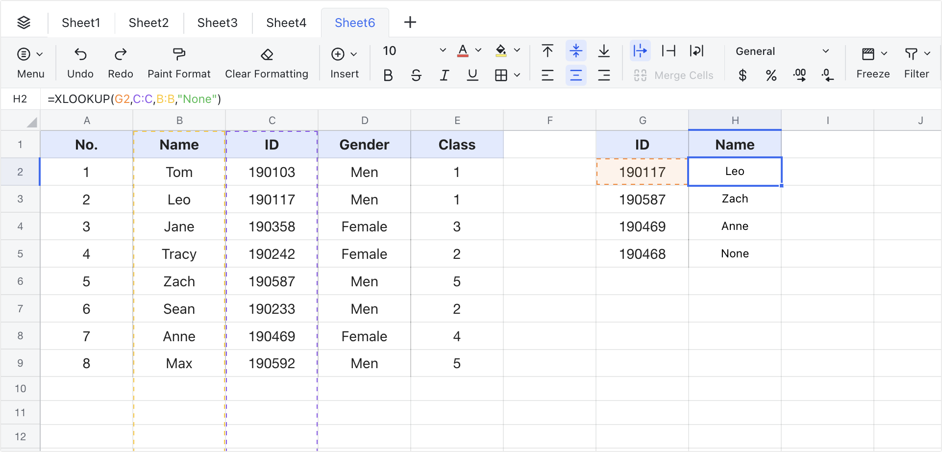
We will use finding a student's name based on their student ID number as an example. The columns A-E in the figure below contains the student's information. We want to search for and return the student's name in column H based on the student ID in column G. If no matching result is found, return "None".
- Open the spreadsheet. Select the H2 cell and enter =XLOOKUP, or click Formulas in the toolbar and select Practical functions > XLOOKUP.
- In the cell, enter =XLOOKUP(G2,C:C,B:B,"None").
- G2 is the lookup value: The value to be searched, here corresponding to the student ID cell 190117.
- C:C is the lookup array: The range to search, which contains the student ID numbers.
- B:B is the return array: The value to return based on the corresponding student ID.
- "None" is the [default return value]: If the name corresponding to the student ID is not found, return "None".
- Press Enter for the results.
- Drag the + icon in the lower-right corner of the cell to other cells as needed.

250px|700px|reset
Use the function across spreadsheets
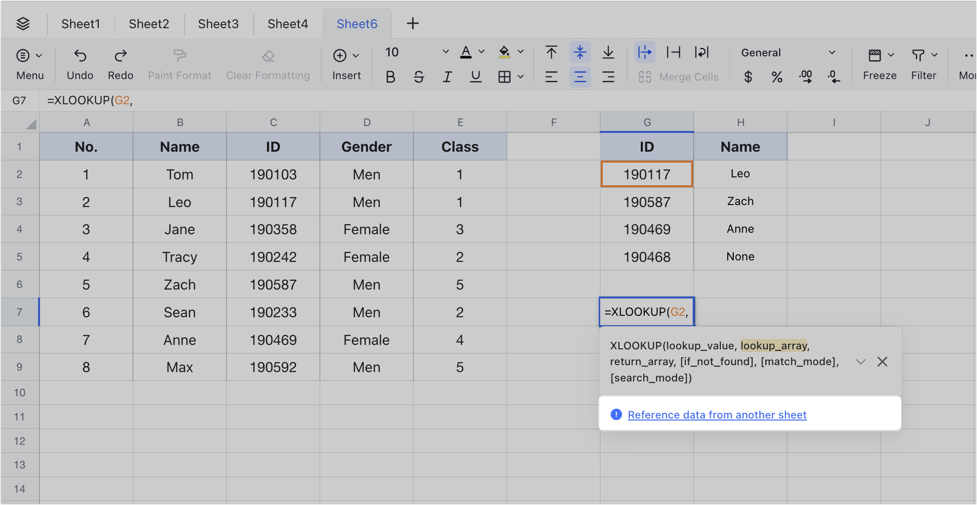
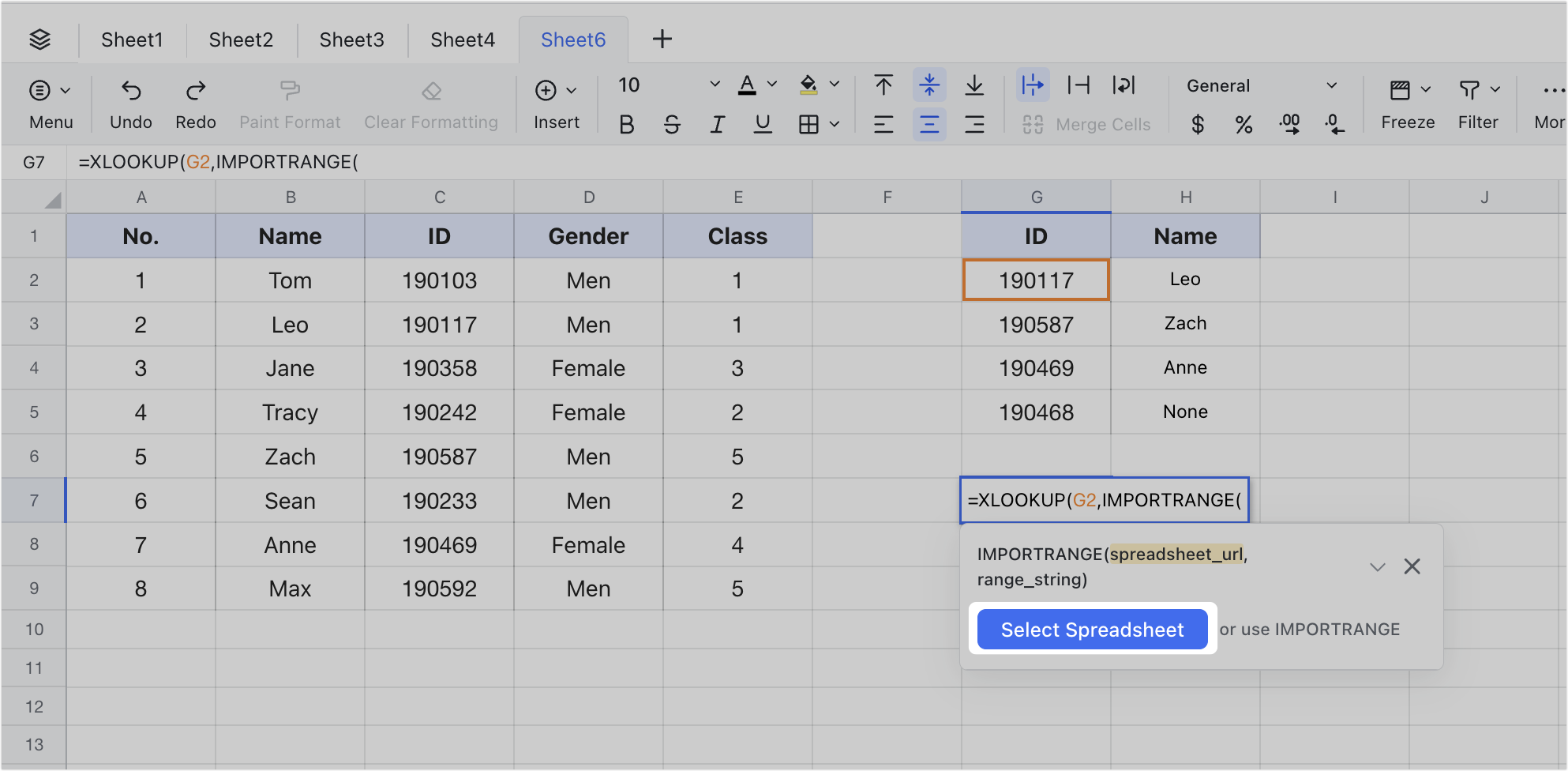
Select a cell and enter =XLOOKUP. Enter the lookup value, and click Reference data from another sheet > Select Spreadsheet to reference data from other spreadsheets for the lookup array and return array as needed.
Note: You can only reference data across spreadsheets once in a formula. If you referenced data for both lookup array and return array in the formula, then the formula will not work.


250px|700px|reset
250px|700px|reset
Delete the function
Select the cell with the XLOOKUP function and press Delete.
IV. Use cases
Determine the grade of exam scores
As a teacher, you'll need to assign grades based on the students' scores. In the figure below, column F contains the scores and G columns contains the corresponding grade. Column C contains the students' actual scores, and we can assign them a grade in column D based on the information in columns F and G. Enter the following formula in cell D2 and drag it down to cell D10.
- Formula used: =XLOOKUP(C2,F:F,G:G,"",-1)
- About the arguments:
- Based on the value in C2, look up the score in column F to find the corresponding grade in column G and return that as the value.
- The fourth argument is set to an empty string "" and cannot be omitted, indicating that if no matching value is found within the lookup array, the function will return an empty string instead of the default "#N/A" error value.
- The fifth argument is -1, indicating that if there is no exact match, the match will be made with the next smaller item. For example, if the lookup value is 37 and there is no exact match in column F, then the match will be made with the next smaller item, which is 0, so"F" is returned. If the lookup value is -1 and there is no exact match in column F, then the match will be made with the next smaller item -100, so "Absent" is returned.

250px|700px|reset
Query the latest sales amount of a product
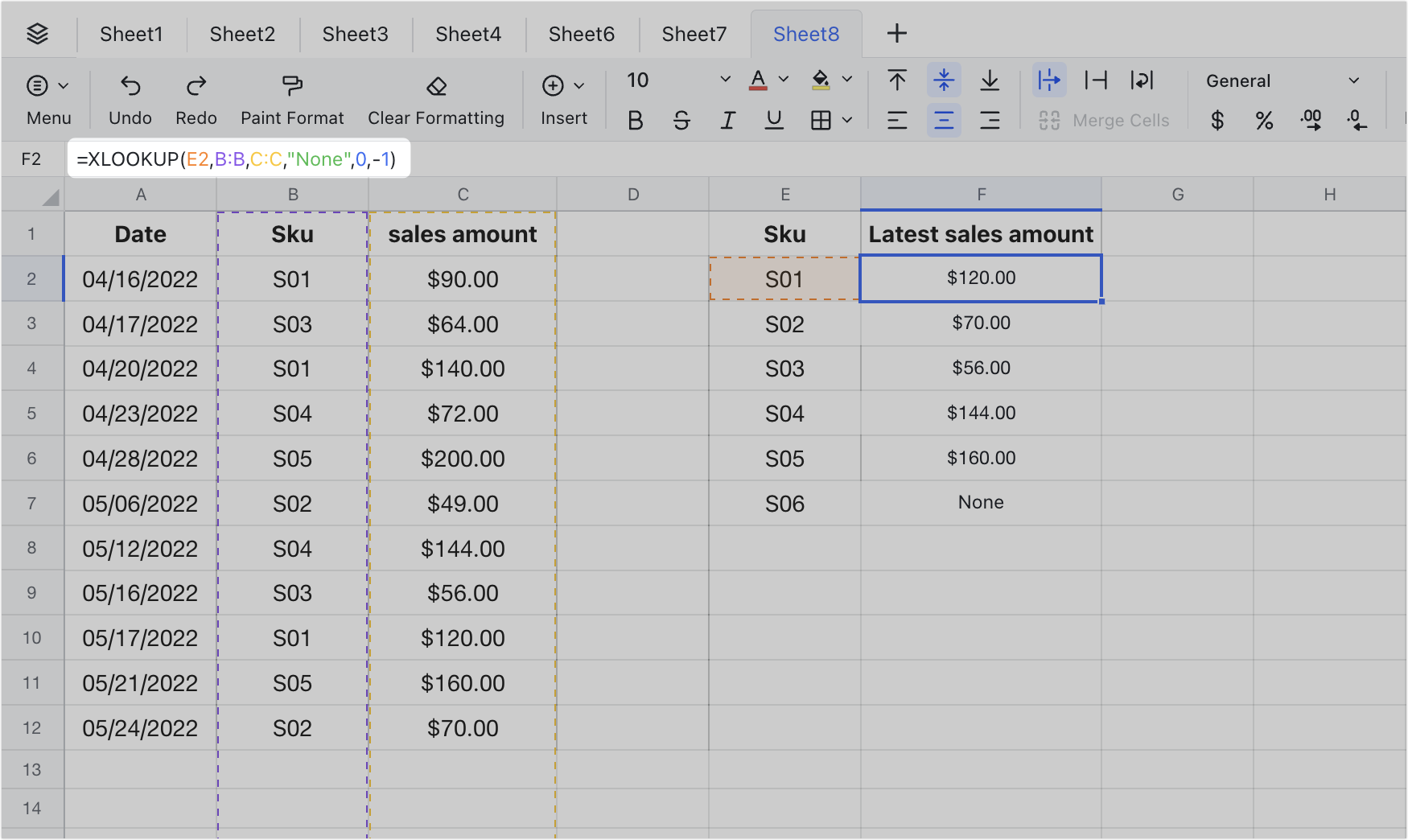
As a sales manager, you may need to know the latest sales amount of a particular product. The A-C columns in the figure below are the sales records of the product, with the dates in column A sorted in ascending order. Enter the following formula in cell F2 and drag it down to cell F7.
- Formula used: =XLOOKUP(E2,B:B,C:C,"None",0,-1)
- About the arguments:
- Based on the value in E2, look up the product in column B to find the corresponding sales amount in column C and return that as the value.
- The fifth argument is 0, indicating that the match mode is exact match.
- The sixth argument is -1, indicating that the search starts from the last item and moves upward. When an exact match is found, the corresponding result is returned. Since the dates are sorted in ascending order, the result returned is the latest sales amount of the product.

250px|700px|reset
