
I. Intro
The AVERAGEIFS function is commonly used to return the average value of a range according to multiple conditions.
II. Explanation
- Formula: =AVERAGEIFS(average_range,range 1,criteria1,[range2,...],[criteria2,...])
- Parameters:
- average_range (required): The range to average.
- range1 (required): The range that will be evaluated by criteria1.
- criteria1 (required): The mode or testing criterion used to evaluate range1. The form of the criterion can be a number, an expression, a cell reference, or text, such as 32, "32", ">32", or B4.
- range2 (optional): Additional ranges to be evaluated.
- criteria2 (optional): Additional criteria to be used for evaluation.
Note:
- Cells in range that contain TRUE or FALSE are ignored.
- If a cell in average_range is empty, then AVERAGEIF will ignore it. If range is empty or contains text values, then AVERAGEIF will return the error value #DIV0!.
- If a cell in criterion is empty, AVERAGEIF will treat it as having the value 0, then AVERAGEIF will return the error value #DIV/0!. In addition, you can use wildcard characters such as the question mark (?) and asterisk (*) in criterion. The question mark matches any single character, and the asterisk matches any strings.
III. Steps
Use the AVERAGEIFS function
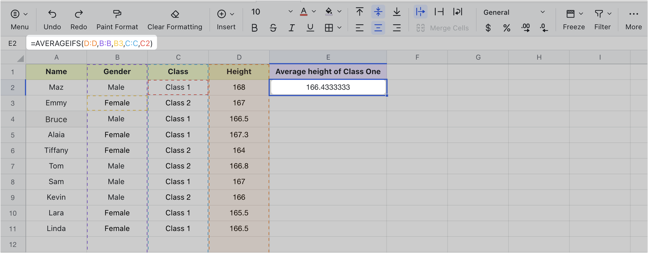
Take calculating the average height of female students in Class 1 as an example. Columns A to D display the student information, where column A is the student's name, column B is the gender, column C is the class, and column D is the student's height.
- Open the Sheets file, select the cell, and enter =AVERAGEIFS in the cell. Or click Formulas on the toolbar. Select Statistics, then select the AVERAGEIFS function.
- Enter formula parameters =AVERAGEIFS(D:D,B:B,B3,C:C,C2) into the cell.
- Press Enter to display the result of 166.4333333 in the cell, which is the average height of female students in Class 1.
250px|700px|reset
Delete the AVERAGEIFS function
Select the cell with the AVERAGEIFS function applied, and press Delete to clear the formula from the selected cell.
IV. Scenarios
Use the AVERAGEIFS function to calculate certain average expenses
Sometimes, people who keep accounts may want to know how much they have spent on a certain commodity. In this situation, they can use the AVERAGEIFS function to set and specify criteria to find their average expenditure for this item.
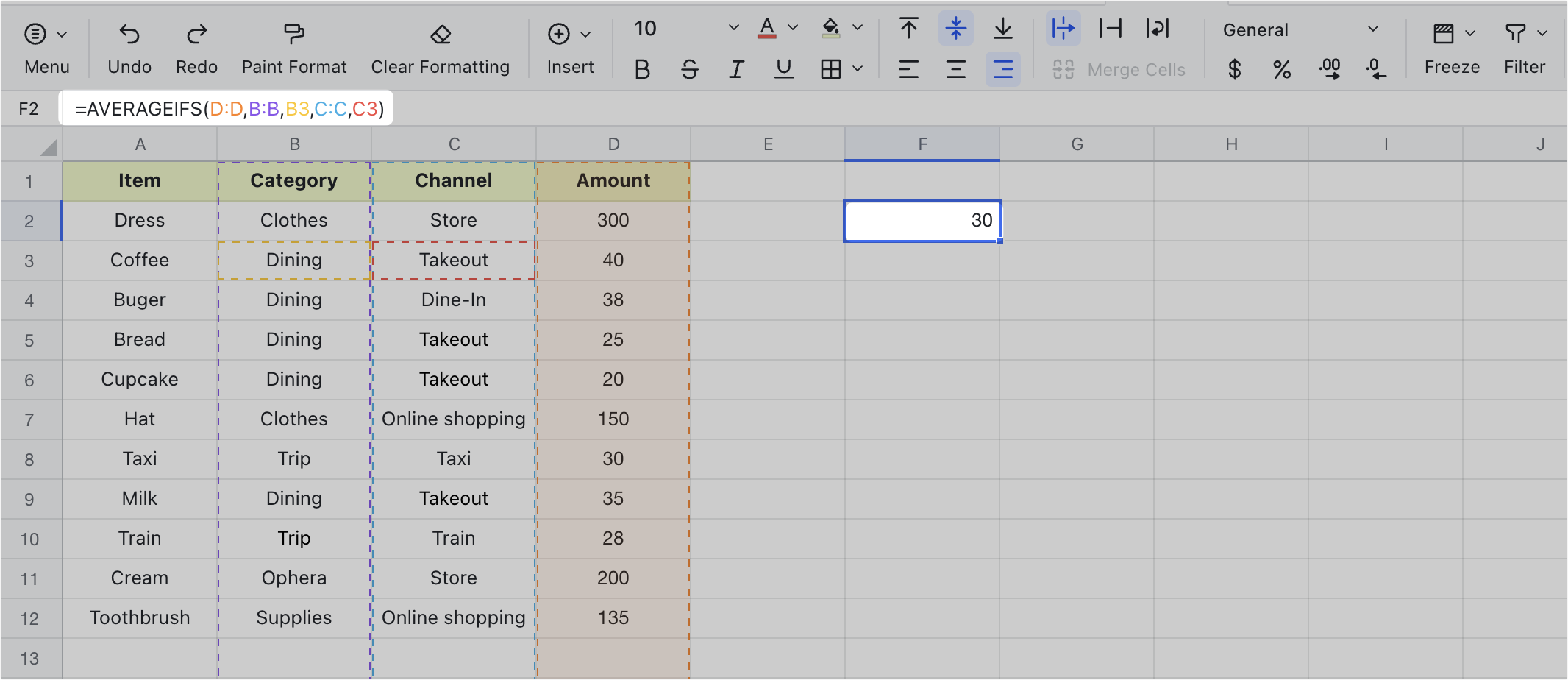
- Formula used in the figure below: =AVERAGEIFS(D:D,B:B,B3,C:C,C3)
- Formula parameter explanation:
- In the figure below, we need to find the average amount spent on takeout. To do this, we first set the range as the Amount column, which is D:D.
- Next, we set criteria1 in column B, which is B:B. Select the "Dining" criterion as the type, then click cell B3.
- Next, we set criteria2 in column C, which is C:C. Select the "Takeout" criterion as the type, then click cell C3.
Press Enter to get the result, which indicates a monthly average of 30 is spent on takeout.
250px|700px|reset