
I. Intro
Pivot table is a tool for sorting and aggregating complex data for advanced analysis. It not only offers summation, counting, averaging, and other calculations, but also provides versatile ways to display key data, enabling you to turn information into insight.
II. Steps
- Create a pivot table
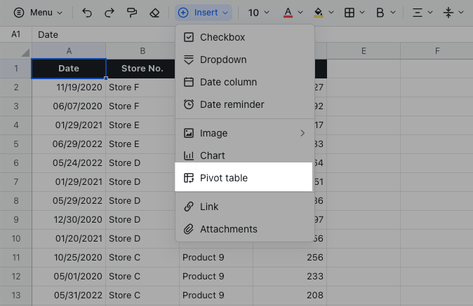
Open the spreadsheet. In the toolbar, click Insert > Pivot table to create a pivot table.
250px|700px|reset
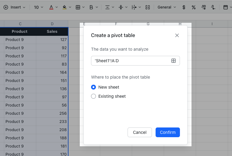
In the pop-up, you can:
- Click the Select a range icon to select the data source. Alternatively, you can select the range that contains the data you want to analyze first, and the selected area will be used as the data source.
- Select the location for the pivot table. If you choose New Sheet, a new sheet with the pivot table will be created. If you choose Existing Sheet, you can add the pivot table into the sheet where the data source is located to make it easier to find the source data.
250px|700px|reset
- Build a pivot table
In the pivot table configuration panel, you can configure the following:
Fields
In the Fields tab, you can directly drag the required fields to different areas of the pivot table.
- Filters: Set which fields you want to filter the data in the pivot table by. For example, dragging the date field into the filter, you can filter out the data of specific dates in the pivot table and the calculation results corresponding to these data.
- Row: Set the value at the beginning of each row in the pivot table. For instance, by dragging the product field into the row area, you can analyze and summarize data in the pivot table by product.
- Column: Set the column name for each column in the pivot table. For example, dragging the region into the column area, you can view the data of products in different sales regions.
- Values: Set the specific indicators to be calculated. For example, by dragging the sales volume into the value area, you can calculate the sales volume of different products in different regions.
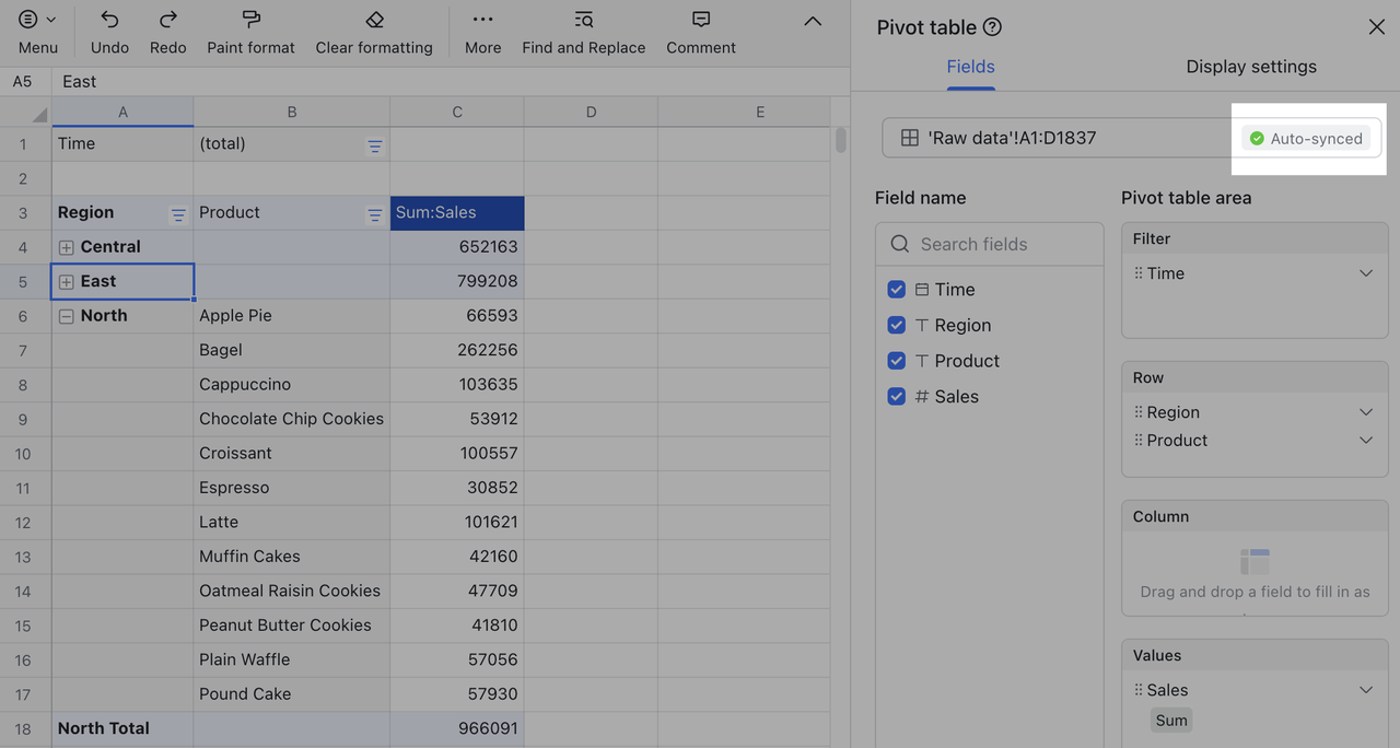
Taking the image below as an example, you can view the total sales volume for each product in different regions, and filter the date to display the total amount at different periods.
250px|700px|reset
Display settings
In the Display settings tab, you can configure the following:
- Show totals: Select the options you need to show subtotals or totals for rows and columns.
- Repeat item labels: Select the options you need to repeat item labels for rows or columns.
- Advanced settings: Select the option to autofit the column width when the data is updated and automatically show pivot table settings as needed. If you don't select the option to automatically show pivot table settings, you can still right-click the pivot table to open pivot table settings.
250px|700px|reset
3. Change the summary method
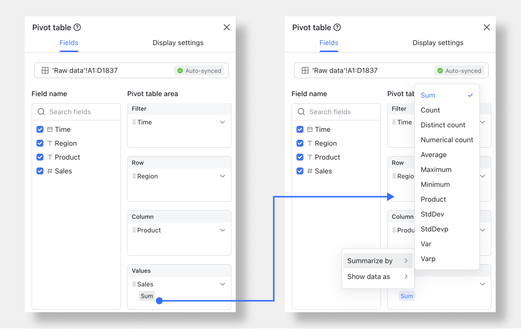
On the Fields tab, you can change how values are summarized and displayed by configuring the summary method and display option.
- Summary method: Click the Gray button below the value > Summarize by to select a summary method the calculation method as needed.
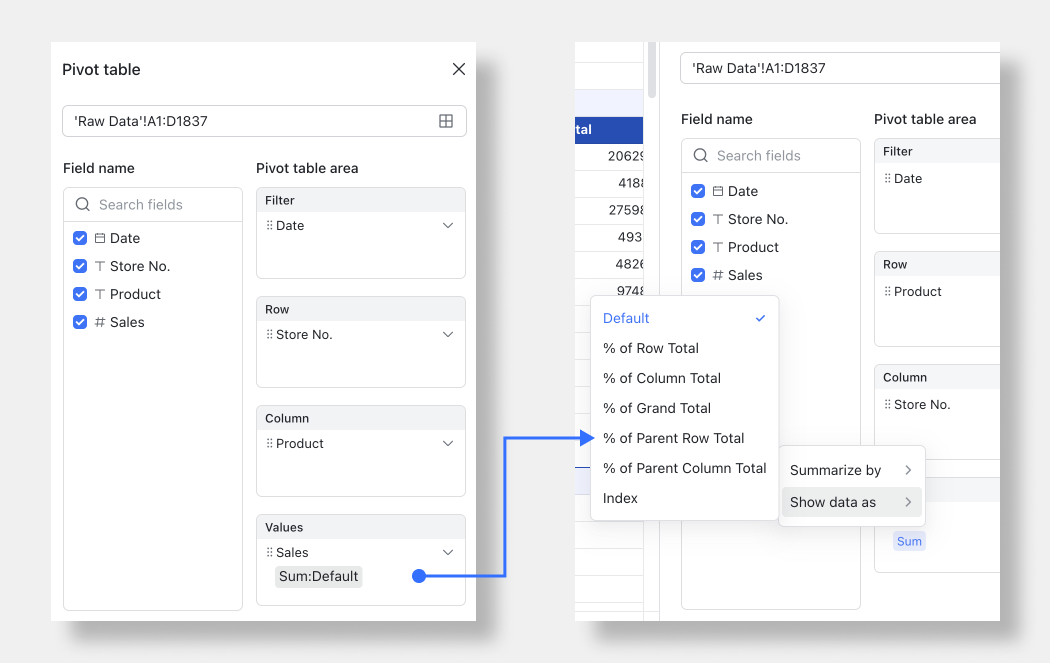
- Display option: click on the Gray button below the value > Show data as to choose how you want the data to be displayed.
250px|700px|reset
250px|700px|reset
- View data in the pivot table
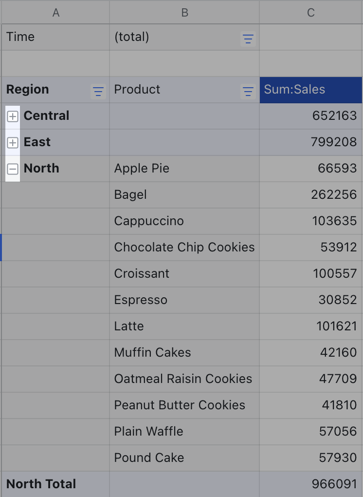
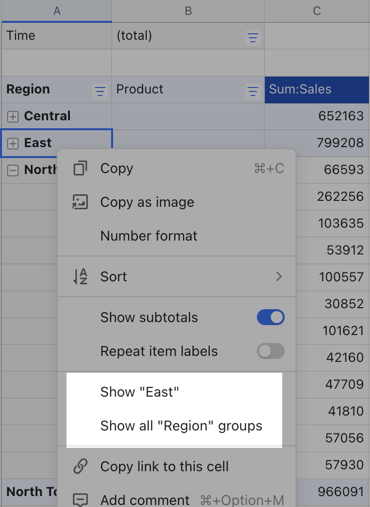
When there are two or more fields in the row or column area, the data will be grouped. Click the + or - icons in front of each group to expand or collapse the group. You can also right-click the cell to expand or collapse the groups. For more details, see Group in pivot tables.
250px|700px|reset
250px|700px|reset
Double-click a cell from the Values field, and the specific entries used for the calculation will be displayed in a new sheet.
250px|700px|reset
5. Update the data source
When the source data changes, but the selected area for the source data has not changed, then the data will sync to the pivot table in real time without the need to be manually refreshed.
If the data source area has changed, it can be modified at the top of the pivot table editing pane.
250px|700px|reset
6. Move the pivot table
You can move the pivot table in any of the following ways:
- Click the cell in the upper-left corner of the pivot table, then hover over the cell border until your cursor becomes a hand, then drag the pivot table.
- Select the entire area of the pivot table, or select any cell and press Ctrl + A (Windows) or Cmd + A (Mac) to select the entire area. Then copy or cut the pivot table and paste it to the target location.
Note: You can't move pivot tables across sheets. If you paste the pivot table to a different sheet, it will become a regular table.
250px|700px|reset
- Delete the pivot table
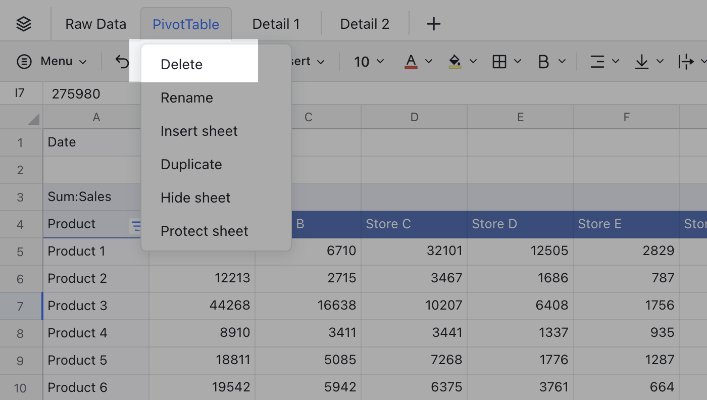
You can delete the pivot table in any of the following ways:
- Click the cell in the upper-left corner of the pivot table and press Delete.
- Right-click the tab of the sheet in which the pivot table is located and select Delete. Note that this deletes the sheet as well as the pivot table.
250px|700px|reset
III. FAQs