I. Intro
The SUMIF function returns the sum of the values that meet the specified criterion in a range.
II. Explanation
- Formula: =SUMIF(range,criterion,[sum_range])
- Parameters:
- Range (required): The cell range that you want to find the sum of.
- Criterion (required): The condition for the range; a cell range with the conditions to be applied.
- Sum_range (optional): The actual area to sum; the cells, area, or reference to be summed. If this parameter is omitted, then the range parameter will be summed.
- Example: =SUMIF(A1:A10,">20",B1:B10)
- Note: Use double quotation marks (") around the criterion.
III. Steps
Use the SUMIF function
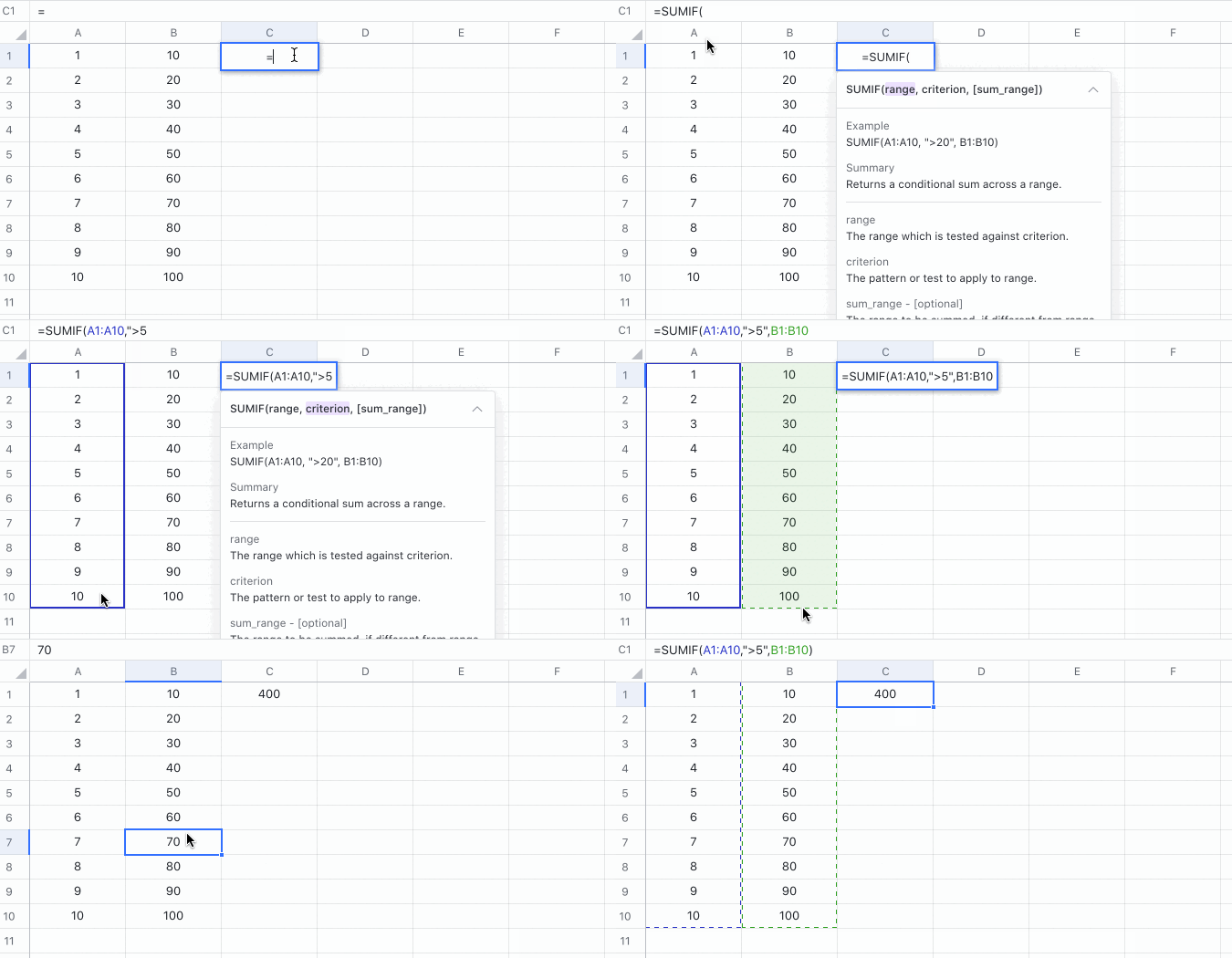
- Select a cell, click Formulas on the toolbar, then select Math > SUMIF. You can also directly enter =SUMIF in a cell.
- Enter the parameters in the cell. For example: =SUMIF(A1:A10,">5",B1:B10).
- Press Enter to display the result, which is 400 in this example.

250px|700px|reset
Delete the SUMIF function
Select the cell with the SUMIF function and press Delete.
