
I. Intro
The TRIMMEAN function is used to find the average, excluding some of the highest and lowest values of the data set. You can use this function if you want to exclude parts of your data from your analysis.
II. About the function
- Formula: =TRIMMEAN(data, exclude_proportion)
- Parameters:
- data (required): The array or range that needs to be sorted and averaged.
- exclude_proportion (required): The proportion of data points to be excluded from the calculation. For example, if exclude_proportion is set to 0.2 in a data set with 10 data points, then 2 will be removed.
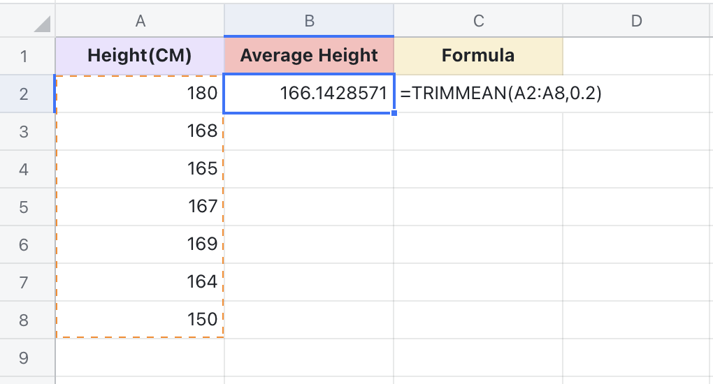
- Example:
- =TRIMMEAN(A2:A8,0.2)
III. Steps
Use the TRIMMEAN function
- Select a cell and click Formulas on the toolbar, then select Statistical > TRIMMEAN. You can also directly enter =TRIMMEAN in a cell.
- Enter the parameters in the cell. For example: =TRIMMEAN(A2:A8,0.2).
- Press Enter to display the result, which is 166.14 in this example.
250px|700px|reset
Delete the TRIMMEAN function
Select the cell with the TRIMMEAN function, and press Delete.
IV. Use cases
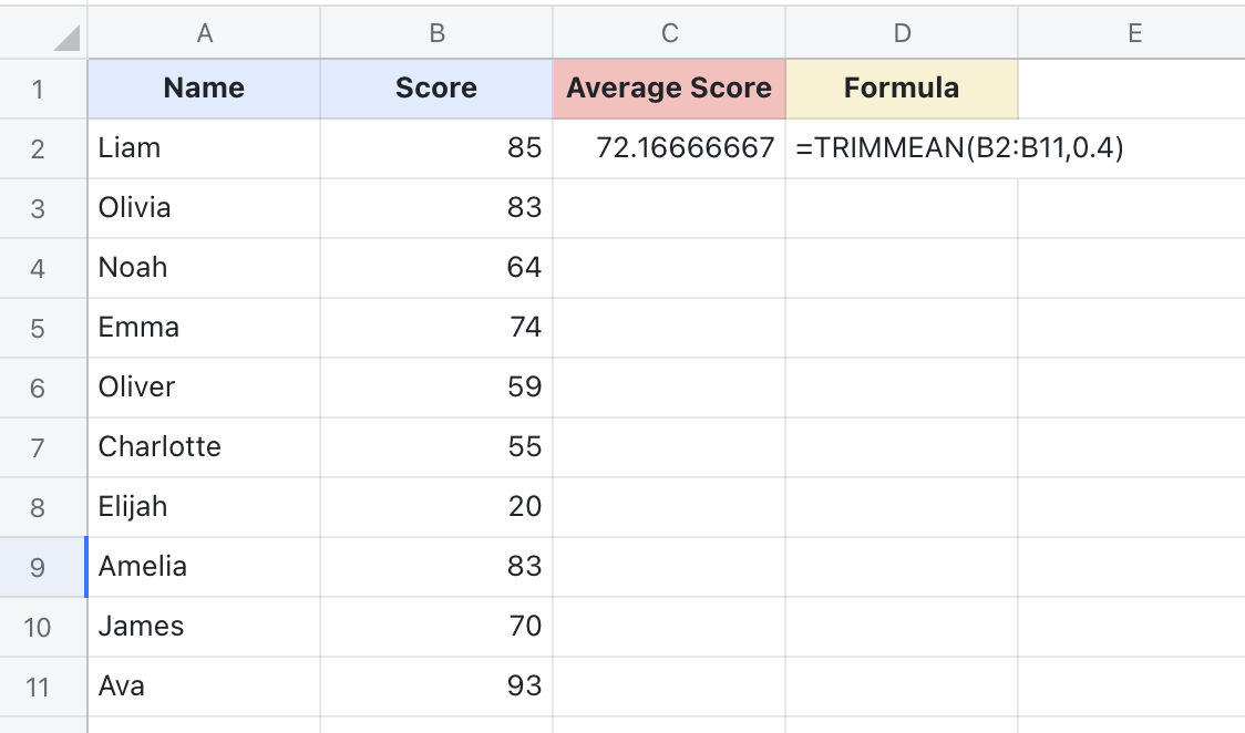
Teachers: Find the average test score
There may be outliers in the class that skews the average. Teachers can use TRIMMEAN to exclude these extreme values (the highest and lowest) to get a more accurate picture of student performance.
- Formula used below: =TRIMMEAN(B2:B11,0.4)
- About the parameters:
- To find a more accurate average, first, check for obvious outliers in the data.
- Select the range containing the data, which is B2:B11.
- Enter 0.4, which removes the four extreme values from this data set of 10. The result is the average of the remaining six values.
250px|700px|reset