
I. Intro
The IFERROR function is commonly used to search for errors in formulas. The function returns the formula result if there are no errors, and returns an error code or specified value if an error is found.
II. About the function
- Formula: =IFERROR(value, value_if_error)
- Arguments:
- value: The formula for which you want to check for errors.
- value_if_error: The value to return if the formula contains an error. If the error return value is text, it needs to be enclosed in double quotation marks.
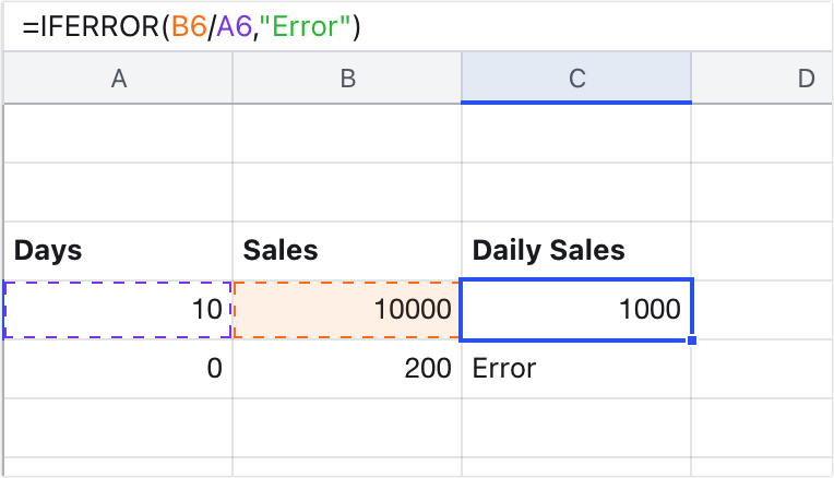
- Example: =IFERROR(B6/A6,"error"), if there is no error in the formula, then the calculation result (Daily sales) will be returned. If the calculation contains an error (such as days being 0), then the word "error" is returned.
250px|700px|reset
III. Steps
Use the function
- Open the spreadsheet, select a cell, and enter the formula =IFERROR(value, value_if_error).
- Press Enter to get the result.
250px|700px|reset
Delete the function
Select the cell with the function and press Delete.
IV. Use cases
Use IFERROR with VLOOKUP
When using the VLOOKUP function, if the lookup value can't be found in the lookup area, an #N/A error will be returned. In this case, you can use the IFERROR function to specify the value to return if an error is found to facilitate subsequent sorting and analysis.
For example, you can use the formula =IFERROR(VLOOKUP(E2,A1:C11,3,0),"Can't find") to find the sales of different employees. If the employee can't be found in the lookup area, it will show that the employee can't be found.
- VLOOKUP(E2,A1:C11,3,0): Find the sales of the employee in the E2 cell from the A1:C11 range.
- IFERROR(VLOOKUP(E2,A1:C11,3,0),"Can't find"): If the employee in the E2 cell from the A1:C11 range, the words "Can't find" will be displayed.
- 250px|700px|reset