
I. Intro
The CHOOSE function is typically used as a filter to find a value argument corresponding to an index value.
II. About the function
- Formula: =CHOOSE(index_value,argument1,[argument2,...])
- Parameters:
- Index_value (required): Index number, can be any integer between 1 and 254. The CHOOSE function returns the corresponding value argument from a list of 1 to 254 value arguments based on the index value, which can be a number, a formula, or a reference to a cell.
- Argument1 (required): A number, cell reference, defined name, formula, function, or text.
- Argument2 (optional): Same as above. Multiple arguments can be specified.
- Example:
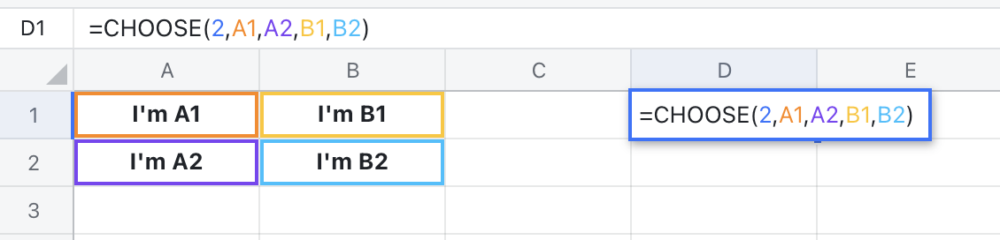
- =CHOOSE(2,A1,A2,B1,B2)
- In this example, of the 4 values in A1, A2, B1, and B2, the second one is selected (A2).
250px|700px|reset
- Note: The value arguments can be range references or single values.
III. Steps
Use the CHOOSE function
- Select a cell and click Formula in the toolbar, then select Search > CHOOSE. You can also directly enter =CHOOSE in a cell.
- Enter the parameters (index_value,argument1,[argument2,...]) in the cell.
- Press Enter to display the result.
250px|700px|reset
Delete the CHOOSE function
Select the cell with the CHOOSE function and press Delete.
IV. Use cases
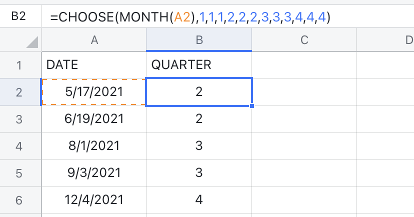
Instantly find a quarter from a date
- About the parameters: This formula involves the use of the MONTH function.
- Formula used below: =CHOOSE(MONTH(A2),1,1,1,2,2,2,3,3,3,4,4,4) calculates that May 17 is in the second quarter.
250px|700px|reset