Use functions in Sheets

7 min read
Audio/video is not supported Please TryRefresh
Play
00:00 / 00:00
00:00
Fullscreen
1x
  • 0.5x
  • 0.75x
  • 1x
  • 1.5x
  • 2x
Click and hold to drag
I. Intro
There is a wide variety of formulas in Sheets to help you make sense of your data. For example: the SUM function can be used to add up numbers, the VLOOKUP function to look for data, and the SUMIF function can be used for adding up items that meet specified conditions.
There are over 500 formulas available in Sheets. For more details, see Data and functions.
II. Steps
  1. To insert formulas in a cell, use the following methods:
Method 1: Directly type the formula in the cell. You will get recommended formulas as you type.
250px|700px|reset
Method 2: Click the cell, select Formulas (or the More icon > Formulas) in the toolbar, and select a formula.
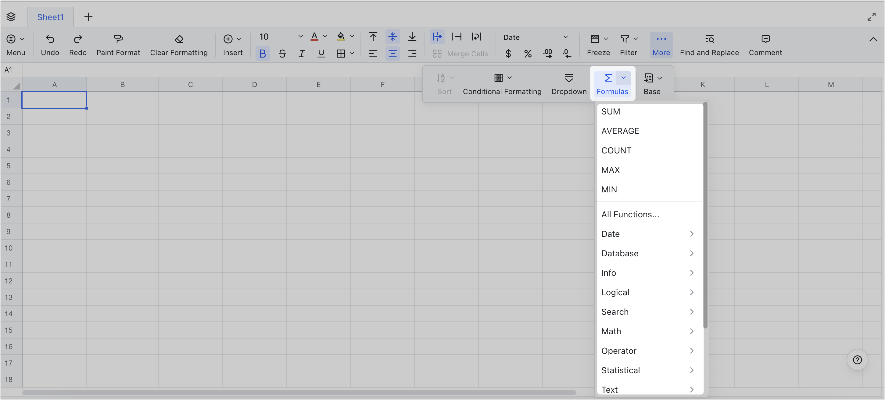
250px|700px|reset
Method 3: Click the cell, click Menu > Data > Formulas, and select a formula.
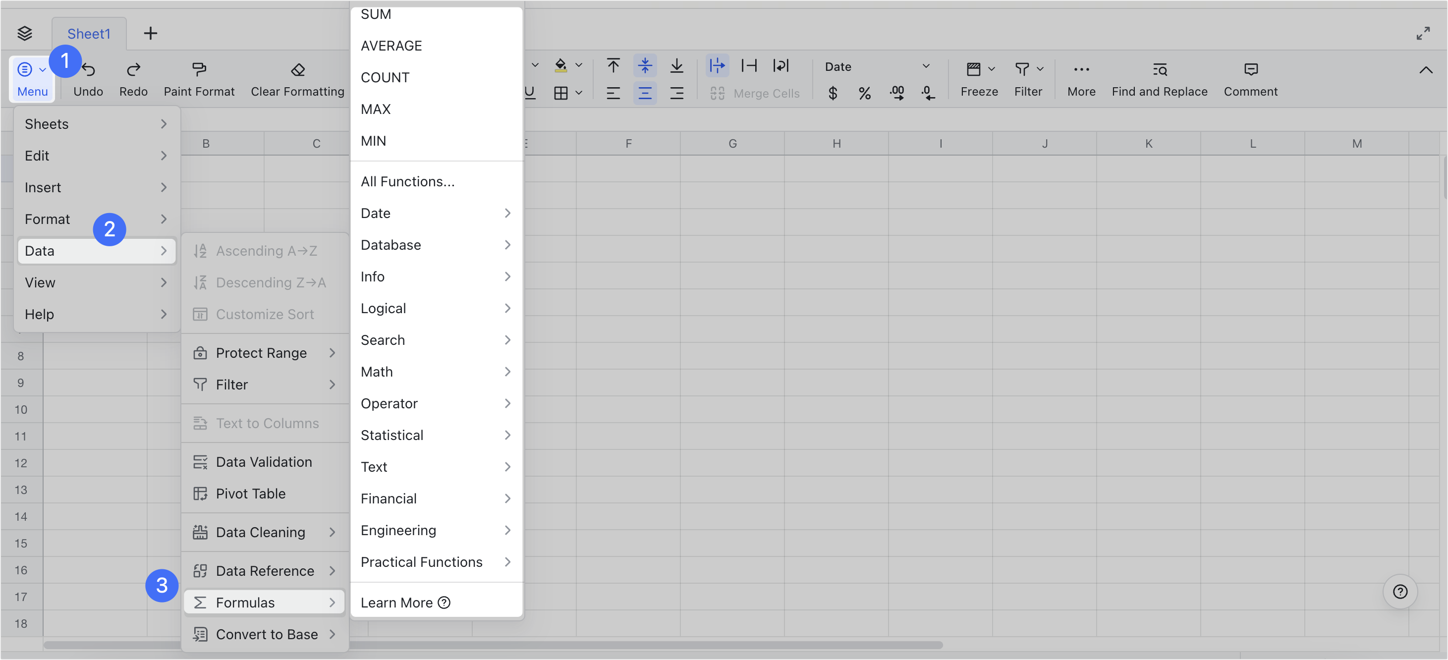
250px|700px|reset
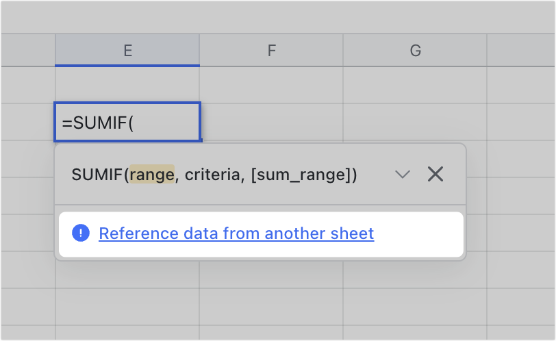
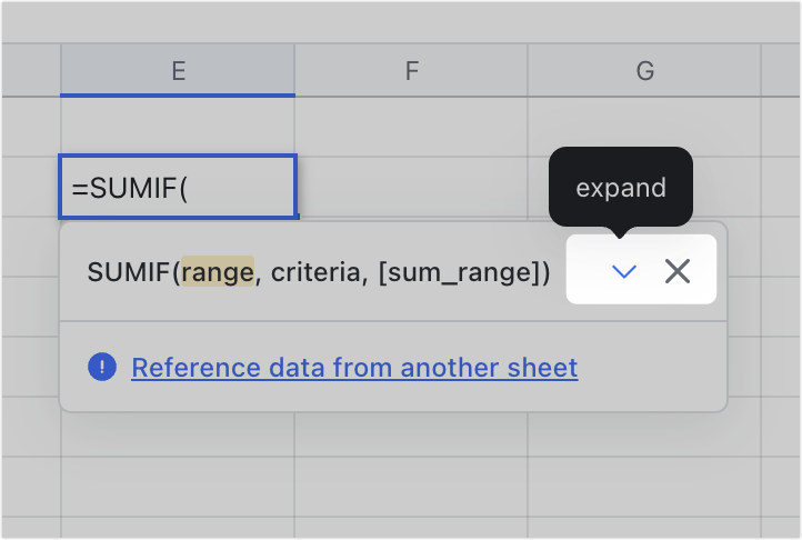
  1. Follow the prompts to enter the arguments, and press Enter to get the results. Click Reference data from other sheets to reference data from other sheets as needed.
Note:
  • Formula prompts are collapsed by default. You can expand it as needed.
  • Arguments in square brackets ([]) are optional, while arguments without brackets are required.
  • Separate each argument with a comma (,). Text content should be enclosed in double quotation marks (").
250px|700px|reset
250px|700px|reset
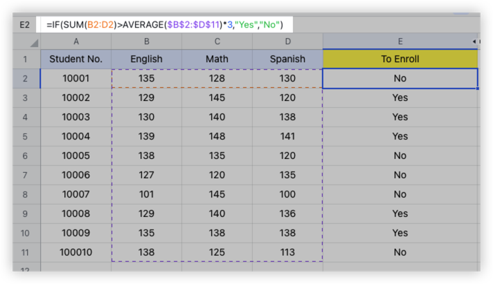
  1. If needed, you can nest multiple formulas in a formula. For example, the table below shows the scores of each subject for students. You can filter out students with total scores above the average score using the IF, SUM, and AVERAGE functions together.
250px|700px|reset
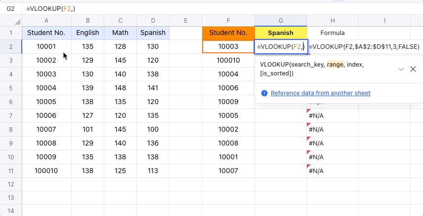
  1. You can apply the formula to other cells by using autofill.
Note that there are two types of references for formulas. If you referenced data in the formula, the returned values will differ depending on the type of reference that is used:
Relative references
The range of data referenced changes with the cell position (this is the default option).
Example: If E2 referenced B2:C2, then E3 will reference B3:C3 when you autofill the formula downwards.
250px|700px|reset
Absolute references
The range of data referenced does not change with the cell position, but is fixed to a specific range. To do this, add the $ symbol(s) to the formula. Example:
  • $D$2 means the cell is fixed (row and column numbers are fixed).
  • D$2 means the row number is fixed, but the column number may change.
  • $D2 means the column number is fixed, but the row number may change.
250px|700px|reset
III. Common errors
If you encounter errors while using functions, you can refer to the following for troubleshooting:
Error
Description
Possible reasons
#NULL!
Empty cell error. This error will appear when you use an incorrect operator in a formula. An example is using a space between two ranges.
  • An incorrect operator is used when referencing ranges in a formula, such as using a space and not a comma or colon.
  • The array size in a formula is inconsistent. An example is the number of rows or columns in two matrices not matching when carrying out a matrix operation.
  • Using an empty cell in a formula.
#DIV/0!
Divisor of zero error. This error will appear when you try to use 0 as a divisor. For example, in =A1/B1, and the value of B1 is 0.
  • The divisor is an empty cell or 0.
  • Certain data is missing in a list or data set, causing 0 to be used as a divisor during calculations.
  • A certain value in the formula is erroneously calculated as 0, causing the division operator to produce an error.
#VALUE!
Value error. This error will appear when you use an incorrect data type under circumstances where it is not permitted. An example is adding text and numbers together.
  • Text and numbers are used for an erroneous operation in a formula.
  • An incorrect data type is used. An example is using a date or time value in a mathematical function.
  • A certain argument in the formula is incorrect. An example is entering an invalid data range.
#REF!
Reference error. This error will appear when you use an invalid cell reference in a formula. An example is deleting a cell referenced in a formula, or using an erroneous cell address in a formula.
  • A cell referenced in a formula has been deleted.
  • An erroneous cell address is used in a formula.
  • A formula containing an invalid reference has been copied or moved.
#NAME?
Name error. This error will appear when you use an undefined name or misspelled function name in a formula.
  • An undefined name is used in a formula.
  • The function name is misspelled.
  • A certain cell reference in a formula is missing quotation marks.
#NUM!
Number error. This error will appear when you use a value that cannot be calculated in a formula. An example is finding the square root of a negative number.
  • A value that cannot be calculated is used in a formula, such as the square root of a negative number.
  • The calculation result of the formula exceeds the value range that can be expressed by the sheet.
  • A certain argument in a formula is not within the permitted value range.
#N/A
Not applicable error. This will appear when a lookup function cannot find a matching value. An example is using the VLOOKUP function to search for a value that does not exist.
  • The search function cannot find a matching value.
  • The data in the data source is incomplete or formatted incorrectly.
  • An incorrect lookup method is used, such as using an incorrect search category in the VLOOKUP function.
#CIRCLE@
Circular reference error. This error will appear when a formula directly or indirectly references the cell it is in. For example, the value of A1 = A1+1.
  • A formula directly references the cell it is in.
  • A formula indirectly references the cell it is in. For example, A1 references B1, and B1 in turn references A1.
  • There is a circular reference between multiple formulas, such that the results cannot be correctly calculated.
IV. FAQs
In Sheets, if I change the format of a cell that contains a formula to "Plain Text", will the formula still work?
No, the formula will no longer work and the formula itself will be shown in the cell.
How do I use a formula to change the data to a percentage in Sheets?
You can use the formula TEXT(cell,"0%") to change a number into a percentage. For example: TEXT(3,"0%")=300%.
How do I enter lowercase "true" or "false" without them being automatically converted to uppercase in Sheets?
Add a space after typing "true" or "false" to prevent them from being automatically converted to uppercase.
How can I reference data from different sheets in a function in Sheets?
When entering the arguments in the formula, follow the prompts to select a different sheet, and then select the data you need.
Written by: Lark Help Center
Updated on 2025-02-05
How satisfied are you with this content?
Thank you for your feedback!
Need more help? Please contact Support.
0
rangeDom
rangeDom
rangeDom
rangeDom
rangeDom