
I. Intro
Platform requirement: These steps can only be performed on the Lark desktop app.
You can reference data from other spreadsheets in Sheets and any updates from the source spreadsheet will be automatically synced to the current spreadsheet. You can reference text, numbers, and formulas, but not links, images, drop-down lists, and data formats.
Use cases:
- For summarizing financial statements, you can reference data across multiple spreadsheets to gather all the relevant data into one single spreadsheet.
- For writing weekly reports, you can reference data from the spreadsheets of different team members to get overall progress for the entire team.
II. Steps
You can reference spreadsheet data in Sheets as well as Docs. The following instructions are for referencing data in Sheets. For referencing data in Docs, see Reference data from Sheets in Docs.
Reference data
Notice: You can only reference spreadsheets for which you have download or copy permission. When you use the data reference feature, the system will automatically check your spreadsheet permissions and create a reference relationship between the spreadsheets.
Open the spreadsheet and reference data using one of the following methods:
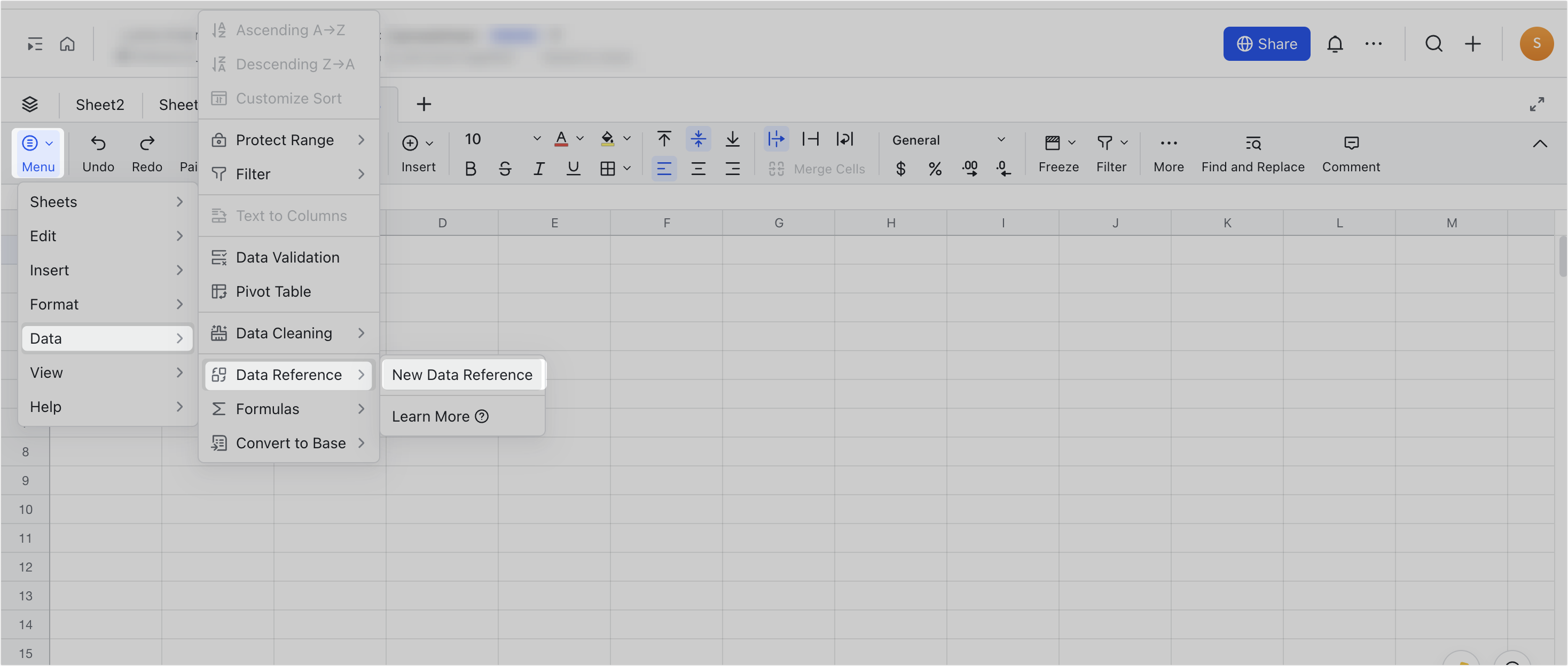
Method 1: Select a cell and click Menu > Data > Data Reference > New Data Reference. In the pop-up window, select the spreadsheet you want to refer to, select the data range, and click Select. Set data format after the data is imported.
250px|700px|reset
Method 2: Enter =IMPORTRANGE and click Select Spreadsheet. Select the spreadsheet you want to reference, select the data range, and click Select. Set data format after the data is imported.
You can also enter =IMPORTRANGE and directly enter the arguments to reference data across spreadsheets. The formula syntax is =IMPORTRANGE(spreadsheet_url, range_string).
250px|700px|reset
Note:
- Up to 100 different data references can be created in one spreadsheet.
- One spreadsheet can be used as a data reference up to 100 times.
- When using cross-spreadsheet data reference in a nested manner, up to 5 layers of nesting are supported. For example, if Sheet B uses the IMPORTRANGE function to reference data from Sheet A across spreadsheets, and Sheet C references data from Sheet B across spreadsheets through the IMPORTRANGE function, this would constitute 3 layers of nesting.
Modify reference settings
After using data reference across spreadsheets, you can adjust the reference settings in three ways: manually updating the data, updating the reference range, or disconnecting the data connection from the source spreadsheet. It may take a few minutes for the adjustment of reference settings to take effect.
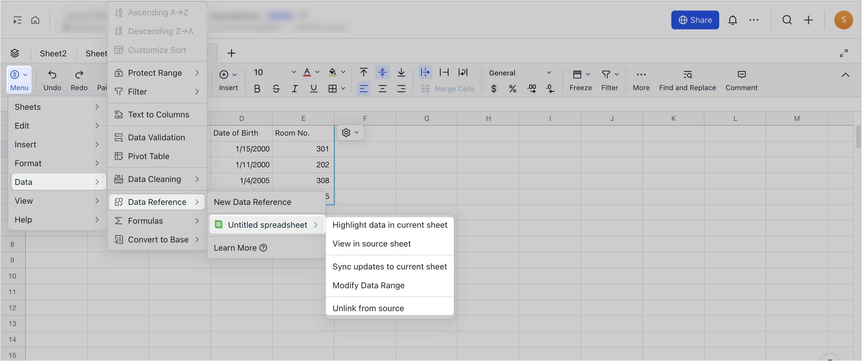
Method 1: Click Menu in the toolbar, then select Data > Data Reference. Select the source spreadsheet and then select a settings option. You can also click Highlight data in current sheet to quickly view data.
250px|700px|reset
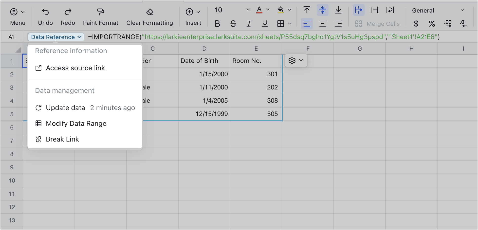
Method 2: Select the cell in the upper-left corner of the referenced data range, click Data Reference from the formula bar, and select a settings option.
250px|700px|reset
Method 3: Click any cell containing the referenced data, click the Settings icon in the upper-right corner, and select a settings option.
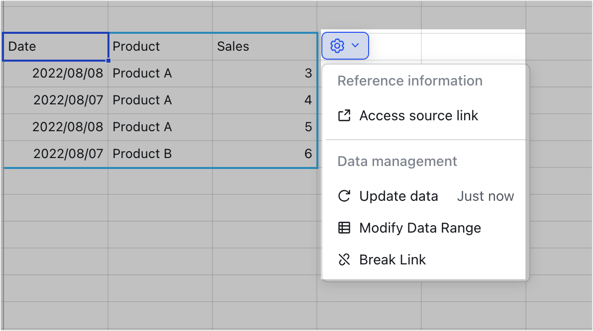
250px|700px|reset
Note: If you modify the reference arguments in the data reference formula, or perform dropdown fill or copy and paste on the cell containing the formula, the system will perform reference and authorization checks again for the action area. #ERROR may be displayed in the cell and you will be prompted to grant permission. At this time, click Grant Permission to proceed.

250px|700px|reset
Delete referenced data
Select the cell in the upper-left corner of the referenced data range and press Delete.
Best practices for data reference
The performance and display of data references in spreadsheets can be influenced by the data within the sheets and the actions performed on them. To optimize the use of the data reference feature across spreadsheets, consider the following recommendations:
- Reduce the number of data references across spreadsheets
- Each data reference across spreadsheets retrieves data from the source spreadsheet. When the source data is modified or the reference function is updated, the system refreshes all reference relationships which can impact performance. Therefore, we recommend you reduce the number of data references across multiple spreadsheets in the formula.
- For example, you can reference the data in the source spreadsheet as a whole instead of referencing them one by one, so as to reduce the number of references.
- As shown in the figure below, column D references the data from A1 to A5 in the source data spreadsheet one by one, using 5 data references across spreadsheets; while column G references the data of the entire area "A1:A5", using only 1 data reference across spreadsheets. At this time, column G has fewer references and is faster.
250px|700px|reset
- Simplify the data range of references
- When other formulas in your spreadsheet depend on the calculation results of data references, calculations will only begin once the data reference calculations are complete. To enhance performance, simplify the reference data range, especially for spreadsheets that are frequently updated or have a large amount of calculations.
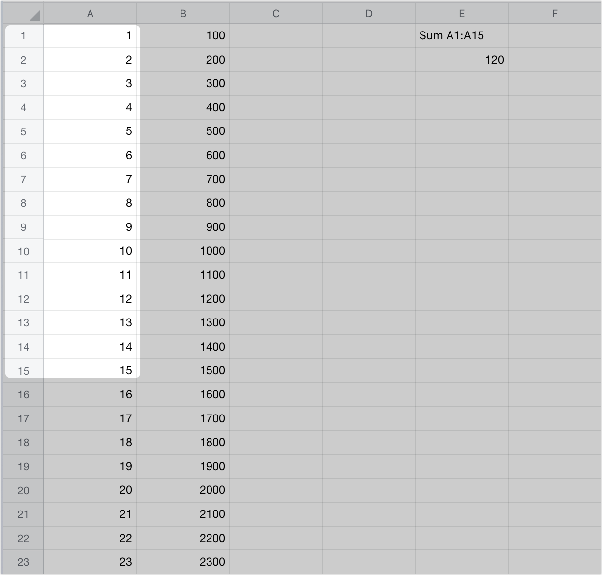
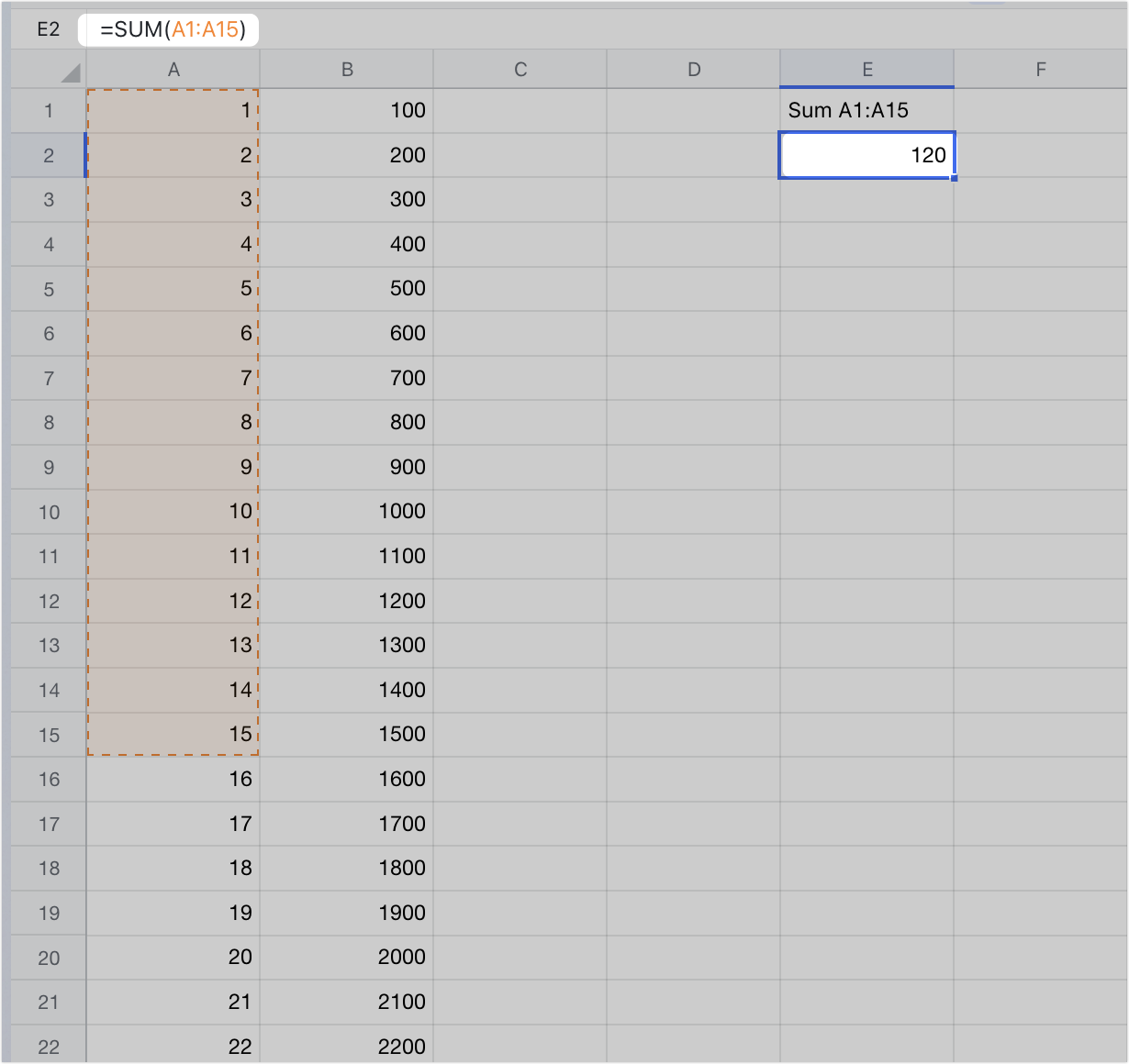
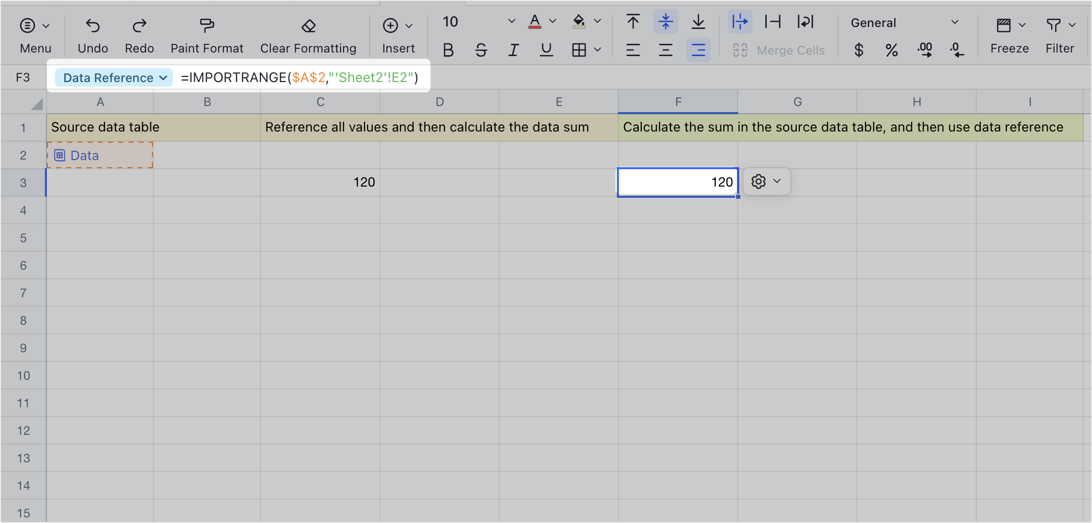
- For example, if you need to calculate the sum of data from A1 to A15 in the source data spreadsheet (as shown in the figure below), you can first calculate the sum in the source data spreadsheet and then use data reference to extract this sum (that is, Method 2), so as to reduce the calculation process between spreadsheets and improve performance.
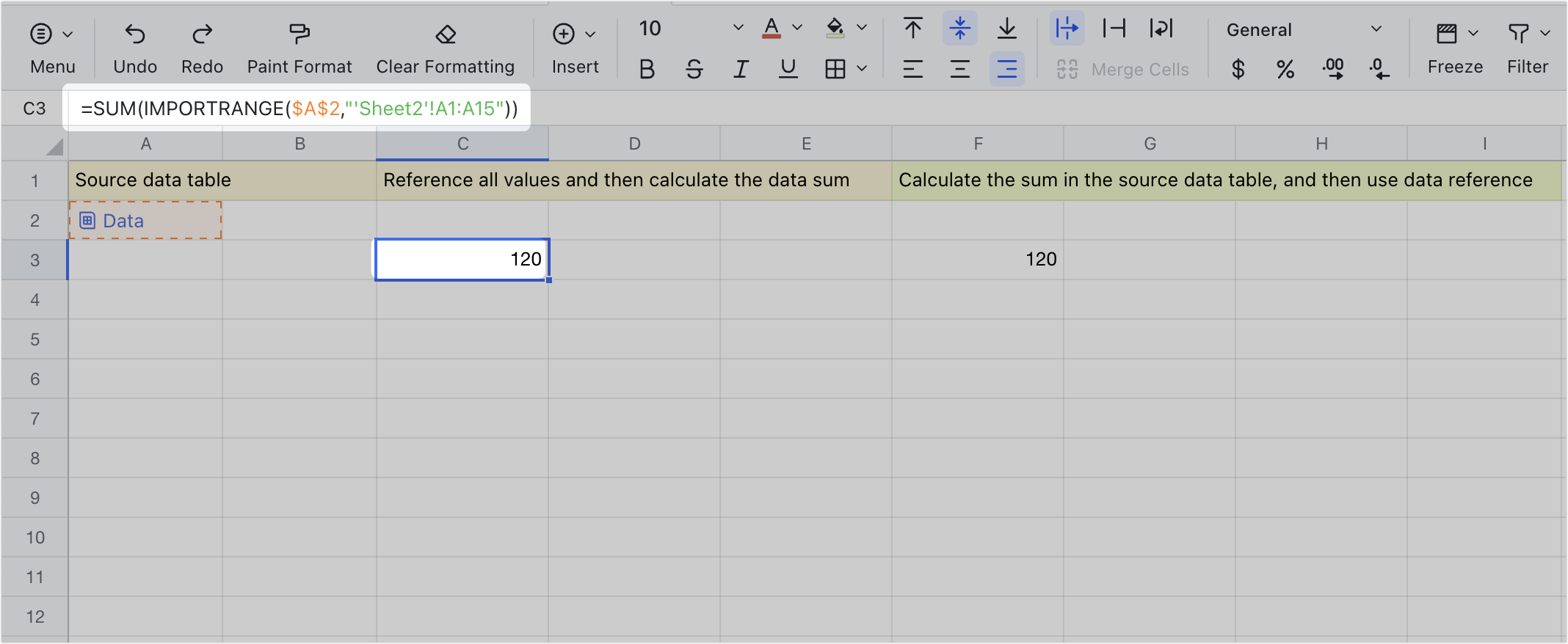
- Method 1: Reference all values and then calculate the data sum, that is, nest the IMPORTRANGE function within the SUM function. Enter =SUM(IMPORTRANGE($A$2,"'Sheet2'!A1:A15")) to obtain a total of 120.
250px|700px|reset
250px|700px|reset
- Method 2 (recommended): First, calculate the sum in the source data spreadsheet (that is, the value of 120 in E2 of the source data on the left), and then use data reference for this data "=IMPORTRANGE($A$2,"'Sheet2'!E2")" to obtain the total of 120.
250px|700px|reset
250px|700px|reset
- Use the IMPORTRANGE chain carefully to avoid creating an IMPORTRANGE loop
- When Sheet B contains IMPORTRANGE(Sheet A) and Sheet C contains IMPORTRANGE(Sheet B), a "chain" is formed. Any updates made to Sheet A will cause Sheets B and C to reload, affecting the performance of IMPORTRANGE. Therefore, we recommend that you:
- Reduce the number of IMPORTRANGE chains formed across multiple sheets. The IMPORTRANGE function nesting supports up to 5 levels.
- Avoid creating an IMPORTRANGE loop. For example, Sheet B contains IMPORTRANGE(Sheet A), and Sheet A contains IMPORTRANGE(Sheet B).
- Avoid using pivot tables and the following functions as arguments for data reference
- It is not recommended to use pivot tables and the following functions as arguments for data reference in Sheets, as frequent updates to these elements may cause data overload. If you need to use pivot tables and the above functions as arguments for data reference, you can copy the calculation results of these functions and then select Paste Special > Paste Values Only to reference a static value for convenient calculation.
-
III. Common error messages
When the system prompts that there is an error in the reference, you can refer to the following situations to troubleshoot the cause of the problem. If the problem still cannot be solved, contact support.
IV. FAQs